Kalman Filter

The Kalman filter assumes variables are random and Gaussian distributed. Each variable has a mean value $\mu$, which is the center of the random distribution (and its most likely state), and a variance $\sigma^2$, which is the uncertainty.

State

• predict the next state (at time $k$) by using the current state (at time $k-1$):
  $\begin{aligned} p_k &= p_{k-1} + \Delta{t} v_{k-1} \\ v_k &= \phantom{p_{k-1} + \Delta{t} } v_{k-1} \end{aligned} \\ \ \\ \begin{aligned} \hat{\mathbf{x}}_k &= \begin{bmatrix} 1 & \Delta{t} \\ 0 & 1 \\ \end{bmatrix} \hat{\mathbf{x}}_{k-1} \\ &= \mathbf{F}_k \hat{\mathbf{x}}_{k-1} \\ \mathbf{P}_k &= \mathbf{F}_k \mathbf{P}_{k-1} \mathbf{F}^T_k \end{aligned} \\$
  • $\mathbf{F}_k$: prediction matrix

Adding external influence

• $a$: external influence (e.g. acceleration)
• $\mathbf{B}_k$: control matrix
• $\vec{\mathbf{u}}_k$: control vector

Adding external uncertainty

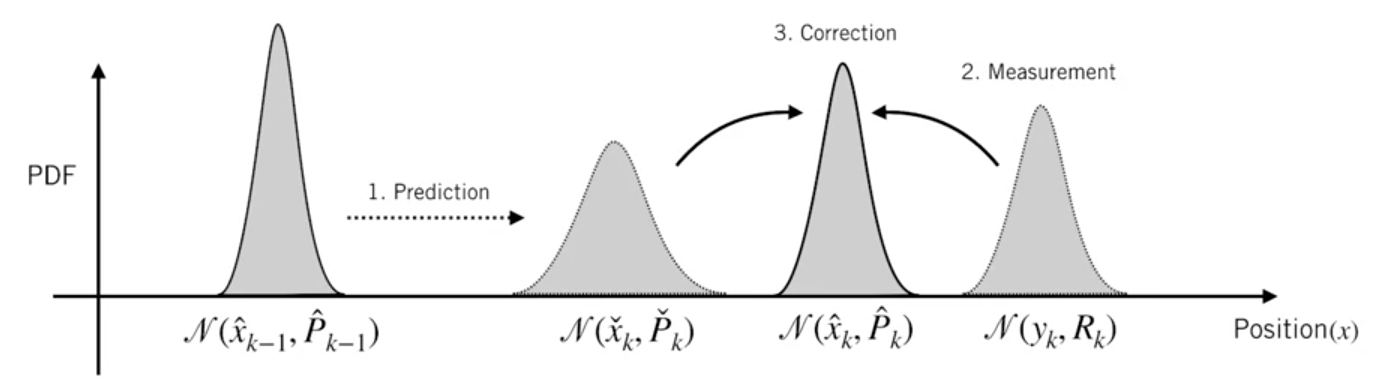
• Prediction step:

  $\begin{aligned} \hat{\mathbf{x}}_k &= \mathbf{F}_k \hat{\mathbf{x}}_{k-1} + \mathbf{B}_k \vec{\mathbf{u}}_k \\ \mathbf{P}_k &= \mathbf{F}_k \mathbf{P}_{k-1} \mathbf{F}^T_k + \mathbf{Q}_k \end{aligned} \tag{1}$
  • $\mathbf{Q}_k$: external uncertainty (noise covariance)
  • The new estimate is a prediction made from previous best estimate, plus a correction for known external influences.
  • The new uncertainty is predicted from the old uncertainty, with some additional uncertainty from the environment.

• Now, we have a fuzzy estimate of where our system might be, given by $\hat{x}_k$ and $\mathbf{P}_k$. What happens when we get some data from our sensors?

Refining the estimate with measurements

• Notice that the units and scale of the reading might not be the same as the units and scale of the state we’re keeping track of. You might be able to guess where this is going: We’ll model the sensors with a matrix, $\mathbf{H}_k$.

• We can figure out the distribution of sensor readings we'd expect to see in the usual way:

  $\begin{aligned} \vec{\mu}_{\text{expected}} &= \mathbf{H}_k \hat{\mathbf{x}}_k \\ \Sigma_{\text{expected}} &= \mathbf{H}_k \mathbf{P}_k \mathbf{H}_k^T \end{aligned}$

• We’ll call the covariance of the sensor noise (uncertainty) $\mathbf{R}_k$. The distribution has a mean equal to the reading we observed, which we’ll call $\vec{\mathbf{z}}_k$.

• So now we have two Gaussian blobs: One surrounding the mean of our transformed prediction, and one surrounding the actual sensor reading we got. We must try to reconcile our guess about the readings we’d see based on the predicted state (pink) with a different guess based on our sensor readings (green) that we actually observed:
  

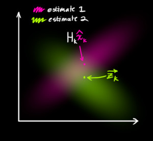
• The Product of Two Univariate Gaussian PDFs is a scaled Gaussian PDF.

  $\mathcal{N}(\mu_0, \sigma_0^2) \cdot \mathcal{N}(\mu_1, \sigma_1^2) = \mathcal{N}(\mu', {\sigma'}^2) \\ \ \\ = \mathcal{N}(\frac{\mu_0 \sigma_1^2 + \mu_1 \sigma_0^2}{\sigma_0^2 + \sigma_1^2}, \frac{\sigma_0^2 \sigma_1^2}{\sigma_0^2 + \sigma_1^2}) \\ \ \\ = \mathcal{N}(\mu_0 + \frac{\sigma_0^2 (\mu_1 - \mu_0)}{\sigma_0^2 + \sigma_1^2}, \sigma_0^2 - \frac{\sigma_0^4}{\sigma_0^2 + \sigma_1^2})$
  • We can simplify by factoring out a little piece and calling it $\mathbf{k}$:
    $\mathbf{k} = \frac{\sigma_0^2}{\sigma_0^2 + \sigma_1^2} \\ \ \\ \begin{aligned} \mu' &= \mu_0 + \mathbf{k}(\mu_1 - \mu_0) \\ \ \\ {\sigma'}^2 &= \sigma_0^2 - \mathbf{k} \sigma_0^2 \end{aligned}$
  • We can extend this formula to matrix version.
    $\mathbf{K} = \Sigma_0(\Sigma_0 + \Sigma_1)^{-1} \\ \ \\ \begin{aligned} \vec{\mu}' &= \vec{\mu}_0 + \mathbf{K}(\vec{\mu}_1 - \vec{\mu}_0) \\ \Sigma' &= \Sigma_0 - \mathbf{K} \Sigma_0 \end{aligned}$
    • $\mathbf{K}$ is called the Kalman gain.
  • As a result, we can take our previous estimate and add something to make a new estimate.

Update step

• We have two distributions: The predicted measurement with $(\mu_0,\Sigma_0)=(\mathbf{H}_k \hat{\mathbf{x}}_k, \mathbf{H}_k \mathbf{P}_k \mathbf{H}_k^T)$, and the observed measurement with $(\mu_1, \Sigma_1)=(\vec{\mathbf{z}}_k, \mathbf{R}_k)$.

• Plug these into above formula.

  $\begin{aligned} \mathbf{H}_k \hat{\mathbf{x}}_k' &= \mathbf{H}_k \hat{\mathbf{x}}_k \ \ \ \ \ \ + \mathbf{K} (\vec{\mathbf{z}}_k - \mathbf{H}_k \hat{\mathbf{x}}_k) \\ \mathbf{H}_k \mathbf{P}_k' \mathbf{H}_k^T &= \mathbf{H}_k \mathbf{P}_k \mathbf{H}_k^T - \mathbf{K} \mathbf{H}_k \mathbf{P}_k \mathbf{H}_k^T \\ \end{aligned} \\$
  • where the Kalman gain is:
    $\mathbf{K} = \mathbf{H}_k \mathbf{P}_k \mathbf{H}_k^T (\mathbf{H}_k \mathbf{P}_k \mathbf{H}_k^T + \mathbf{R}_k)^{-1}$

• We can knock an $\mathbf{H}_k$ and an $\mathbf{H}_k^T$ off the front and the end of terms properly.

  $\begin{aligned} \hat{\mathbf{x}}_k' &= \hat{\mathbf{x}}_k + \mathbf{K}' (\vec{\mathbf{z}}_k - \mathbf{H}_k \hat{\mathbf{x}}_k) \\ \mathbf{P}_k' &= \mathbf{P}_k - \mathbf{K}' \mathbf{H}_k \mathbf{P}_k \end{aligned} \tag{2}$
  $\mathbf{K}' = \mathbf{P}_k \mathbf{H}_k^T (\mathbf{H}_k \mathbf{P}_k \mathbf{H}_k^T + \mathbf{R}_k)^{-1} \tag{3}$

• $\hat{\mathbf{x}}_k'$ is our new best estimate. We can go on and feed it (along with $\mathbf{P}_k'$ ) back into another round of predict or update as many times as we like.

Of all the math above, all we need to implement are equations $(1)$, $(2)$, and $(3)$.

---

📙 참고

• Bzarg - How a Kalman filter works, in pictures
• University of Toronto - State Estimation and Localization for Self-Driving Cars