RSDP_Image Processing

An image is represented by matrix.
In conclusion, image processing is nothing more than changing the element values of matrix.

Image enhancement

• Brightness, contrast enhancement
• Denoising
• Deblurring

Image Transform

• Geometric transform
• Frequency domain
• Hough transform

Image Restoration

• Colorization
• Inpainting

Pixel Point Processing

픽셀 단위로 전부 동일한 연산을 적용 하는 것.

Result

• Shape is fixed.
• Pixel values are more important than their positions.
• Only pixel values relatively changes.

이 경우, 픽셀의 위치보다는 픽셀 값 자체가 중요하다.
input : 픽셀 값

모든 픽셀들이 개별적으로 연산이 된다.

Simple method

• y = T(x) , T is a linear mapping function.

Contrast

콘트라스트 (대비) : 가장 밝은 부분과 가장 어두운 부분의 차이

• an brightness difference between two or more things.
• Various methods to adjust contrast
  (linear mapping, exponential, gamma correction, histogram equalization)

L'(x,y) = aL(x,y) + b

1. b > 0 일 때

그냥 전체적으로 사진이 밝아진다.

2. a > 1 일 때

콘트라스트가 커져서 사진이 선명해진다.

Non - linear mapping function : Gamma function

감마 (r) > 1 일 때는 exponential 형태를 띠고,
r < 1 일 때는 log 함수의 형태를 띤다.

이때 I 는 0~1 사이의 값이어야 한다.

따라서 , 감마 function 을 적용할 때는

I (범위 : 0~255) 를 255 로 나누어서 0~1 사이의 값으로 만들어준 후, r 승을 하고 이후 255 를 곱해주어 원래의 값으로 복원한다.

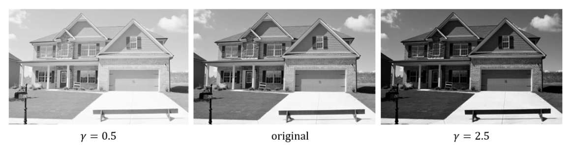
다음 사진에서 감마 값이 1보다 작을 때는 contrast 가 낮아지고, 1보다 크면 contrast 가 커지는 것을 확인할 수 있다.

교수님께서 주신 코드

import numpy as np
import cv2 as cv

#  영상을 로딩하여 numpy array로 저장합니다.
img = cv.imread('zip.png', 1)

# color 영상을 gray scale로 바꿔줍니다.
gray = cv.cvtColor(img, cv.COLOR_BGR2GRAY)
new_gray = np.zeros(gray.shape, gray.dtype)

# 잘되었는지 출력 한번 해봅니다.
cv.imshow("gray image", gray)

gamma = 2.0

# 이론을 그대로 적용한 방법
# 모든 픽셀들 각각에 대해서 값을 변경해줍니다.
# shape[0]: 이미지의 높이(H)
# shape[1]: 이미지의 너비(W)
# matrix를 indexing 할때는 Row, Column순서로 지정합니다. gray(3,5) 는 3행 5열을 뜻합니다.
for y in range(gray.shape[0]):
    for x in range(gray.shape[1]):
        new_gray[y,x] = np.clip((gray[y,x] / 255.0) ** gamma * 255.0, 0, 255)

# 어찌 변환되었는지 출력 한번 해봅니다.
cv.imshow("gamma correction", new_gray)


# 키 입력이 있을 때까지 기다립니다.
cv.waitKey(0)

color conversion

gray = 0.299R + 0.587G + 0.114B

초록색이 실제로 가장 밝고, 그 다음이 붉은색이므로 가중치를 두어서 Grayscale 로 변환한다.

gray = cv.cvtColor(img, cv.COLOR_BGR2GRAY)

Image Transform

Fourier Transform

Main Idea : Any periodic function can be decomposed into a summation of sines and cosines.
Mathematically easier to analyze effects of transmission medium, noise , etc. on simple sine function , then add to get effect on complex signal.

세상의 모든 복잡한 신호들을, 간단한 신호들의 합으로 나타낼 수 있다.

• Fourier transform
  Convert continuous signals of time domain into frequency domain.

• Inverse Fourier transform
  Converse continuous signals of frequency domain into time domain.

• Discrete Fourier transform (DFT)
  The equicalent of the contiuous Fourier fransform for discrete (sampling) signals.

• Fast Fourier transform (FFT)
  A fast algorithm for computing the Discrete Fourier Transform.
  In image processing, FFT is mainly used.

Fourier Transform is invertible.

Frequency on images

영상에서 frequency 라는 것은 무엇인가?

• high frequency : edges, points
• low frequency : All the rest

Image Restoration

Removing artifacts by frequency analysis.

Types of artifacts:

1. Noise
2. Unwanted pattern

Methodology:

1. Convert image to frequency domain using FFT.
2. Remove Artifacts.
3. Convert frequency values to image using iFFT.

교수님께서 주신 코드_FFT_deniosing

import numpy as np
import cv2 as cv

# 그림을 읽습니다.
img = cv.imread('noisy.jpg',0)

# FFT 수행
f = np.fft.fft2(img)
# 기본적으로 fft2를 수행하면 low frequency가 가장자리가 됩니다. 이들을 중앙으로 flip 하기 위해 fftshift를 사용합니다.
fshift = np.fft.fftshift(f)
img_fft = 20*np.log(np.abs(fshift))

# 중앙 값을 구해서 정수로 변환합니다.
[h, w] = img_fft.shape
hh = np.int(h/2)
ww = np.int(w/2)

#  remove outer region
filter_size = 40
fshift_denoising =np.zeros(fshift.shape, fshift.dtype)
fshift_denoising[hh-filter_size:hh+filter_size, ww-filter_size:ww+filter_size] = \
    fshift[hh-filter_size:hh+filter_size, ww-filter_size:ww+filter_size]
img_fft_denoising = 20*np.log(np.abs(fshift_denoising)+1)


# inverse fft
f_ishift = np.fft.ifftshift(fshift_denoising)
img_back = np.fft.ifft2(f_ishift)
img_back = np.real(img_back)

cv.imshow('original', img)
cv.imshow('FFT_before', img_fft/1000)
cv.imshow('FFT_after', img_fft_denoising/1000)
cv.imshow('denoising', img_back/255)

cv.waitKey(0)

Hough Transform

Convert (x,y) domain to ($\rho,\theta$) cordinate.

represent a line on (x,y) coordinate to a point on the ($\rho,\theta$) cordinate.

허프 변환은 line 을 point 로 변환한다.

마치 y = ax + b 라는 선을 앞의 계수만 따서 (a,b) 로 표시할 수 있는 것 처럼...

Hough transform is used for detection certain shapes (especially lines)

1. Suppose that there is a point p(x,y)
2. Infinitely many straight lines pass through that point.
3. Each line can be represented to a point in ($\rho,\theta$) coordinate.
4. Lines passing through p(x,y) are represented in th form of a curve.
5. The straight line we are looking for appears as a superposition (such as a point ) of the curves in A.

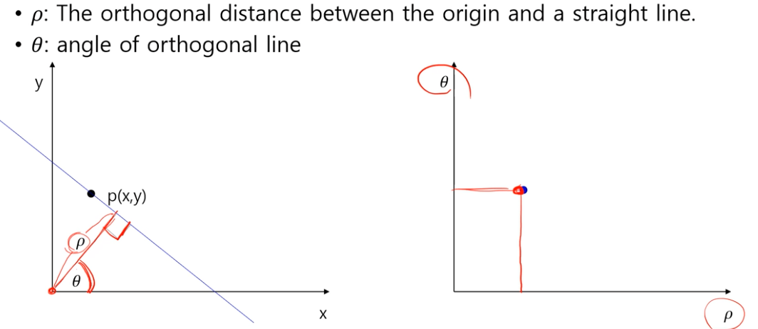
어떤 직선이든지 그 직선에 수직인 직선을 그릴 수 있고,
점과 직선 사이의 거리 (rho) 와 그 각도 (theta) 를 알 수 있고,

이 두 값을 basis 로 하는 새로운 좌표계를 만들어서 좌표계에 그 값에 해당되는 위치에 점을 찍을 수 있다.

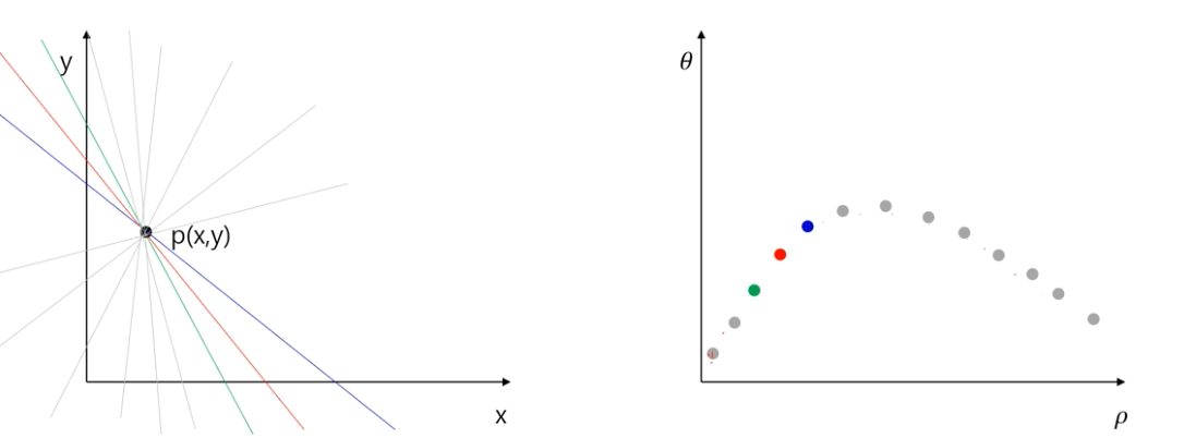
일정한 각도로 선을 회전하면 그에 맞는 rho 와 theta 가 새로 생기고, 점들을 찍으면 다음과 같이 곡선이 나타난다.

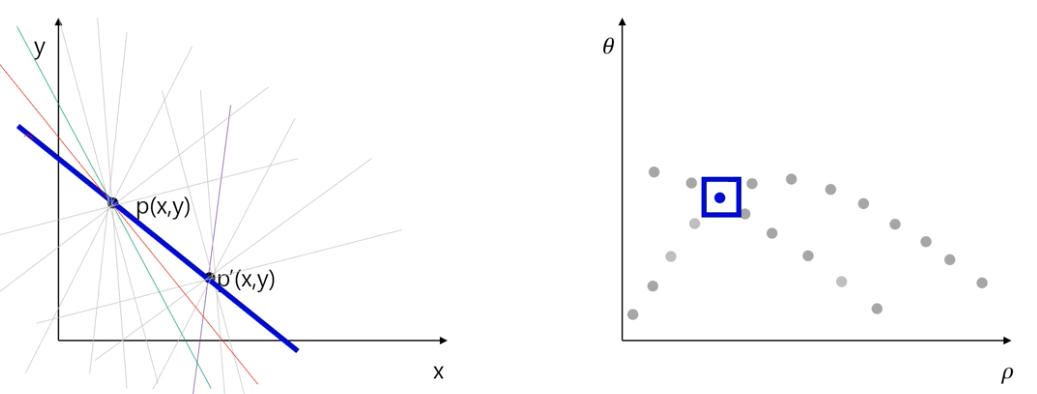
또 다른 점을 찍어서 동일한 과정을 거쳤을 때, 겹치는 점이 의미하는 것은 p점과 p' 점을 동시에 지나는 직선이다.