1. Introduction

• LLM is not guaranteed to be accurate for all queries

• Understanding which queries they are reliable for is important

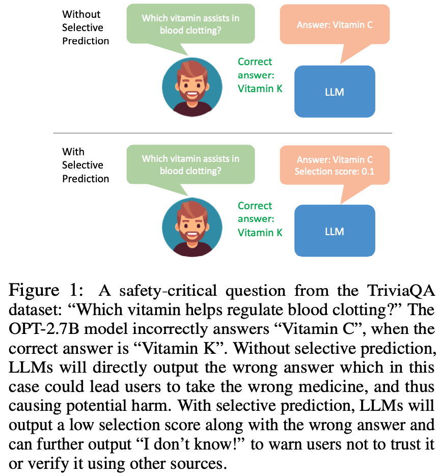
• Selective Prediction : the deployment scenario for AI where humans are involved to maintain overall accuracy by reviewing AI-generated, low-confidence outputs

  • Both human and AI performance are considered together to minimize human involvement cost
  • AI should use Selective Prediction to assess the accuracy of their prediction and refrain from making wrong predictions
  • Able to say "I don't know" when its prediction is not confident

• Selective Prediction is hard as LLM is trained to predict not the "correct" next token but only the "next" token

• It doesn't generate a confidence score also $\rightarrow$ obtaining confidence score from output sequence is not straightforward

• Distinguishing the correctness from likelihood scores is a challenging

  • Using Prompt (Is the proposed answer True or False?) $\rightarrow$ not generalized to other LLMs
  • Semantic Entropy or Self-consistency $\rightarrow$ should generate multiple output sequence
  • Fine-tuning LLMs on target question can improve the likelihood of the ground-truth $\rightarrow$ it is not same as minimizing wrong answers and it still has probability to generate wrong answers

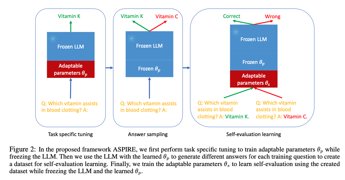
• ASPIRE : learns self-evaluate from target-task data

  • training LLMs on a subset of the training data from the QA tasks
  • define a selection score that combines the likelihood of the generated answer with the learned self-eval score to make selective predictions
  • less computationally expensive than generating multiple output sequences

2. Related Work

Selective Predictions for LLMs

• Selective Prediction for classification (NLI) vs Selective Prediction for NLG
  • NLG task has infinite size of the possible answer set
• Uncertainty Measure for LLMs
• Use selective prediction to solve QA task when question is ambiguous
• Use auxiliary model to distinguish correct predictions of QA model

Parameter Efficient Fine-Tuning (PEFT)

• LoRA
• Prefix Tuning
• Soft Prompt Tuning $\rightarrow$ used!
• P-Tuning

3. Problem Setup

Notations

• pretrained LLM $f$ for arbitary generative modeling task like QA
• vocabulary $\mathcal{V}$
• the space of sequences of tokens $\mathcal{V}^*$
• logits of $f$ on $v \in \mathcal{V}$ given $\mathbf{x} \in \mathcal{V}^*$ is $\bar{f}(v \ | \ \mathbf{x})$
• the likelihood of the next token following $\mathbf{x}$ being $v$ is
  $f(v \ | \ \mathbf{x}) := {\exp(\bar{f} (v \ | \ \mathbf{x})) \over \sum _{v' \in \mathcal{V}} \exp (\bar{f} ( v' \ | \ \mathbf{x}))}$
  (softmax!)
• likelihood of generating $\hat{\mathbf{y}} \in \mathcal{V}^*$ given $\mathbf{x}$ is
  $f(\hat{\mathbf{y}} \ | \ \mathbf{x}) := \prod_{i=1}^{|\hat{\mathbf{y}}|}f(\hat{y_i} \ | \ \mathbf{x}, \hat{y}_{[i-1]})$
  where $\hat{\mathbf{y}} = (\hat{y_1}, \hat{y_2}, ... \hat{y}_{|\hat{\mathbf{y}}|})$ and $\hat{y}_{[i-1]} = (\hat{y_1}, ... \hat{y}_{i-1}), \hat{y}_{[0]} = \empty$
• This likelihood can be very small when $|\hat{\mathbf{y}}|$ is very large $\rightarrow$ normalize the likelihood
  $f_{\text{norm}}(\hat{\mathbf{y}} \ | \ \mathbf{x}) := f(\hat{\mathbf{y}} \ | \ \mathbf{x})^{{1 \over |\hat{\mathbf{y}}|}}$
• use $f$ to generate the output sequence by solving
  $\hat{\mathbf{y}} ^ * = \argmax_{\hat{\mathbf{y}}} \log f(\hat{\mathbf{y}} \ | \ \mathbf{x})$
• Impossible to solve exactly as the output sequence is arbitrarily long $\rightarrow$ use decoding strategy (greedy decoding, beam search) to solve it

Evaluate Correctness

• set of reference outputs $S$

• evaluation metric $M : \mathcal{V}^* \times \mathcal{V}^* \rightarrow \ [0,1]$

  • evaluate the similarity of the generated output $\hat{\mathbf{y}}$ and the reference output $\mathbf{y}_r \in S$

• threshold $\gamma$

  • if $\max_{\mathbf{y}_r \in S} M(\hat{\mathbf{y}}, \mathbf{y}_r) > \gamma$, then the generated output is correct

• training dataset $\mathcal{D}^{tr} = \{ (\mathbf{x}^i, S^i) \}_{i=1}^{n_{tr}}$ randomly sampled from a target task distribution

• rejection operation $\bot$

• selective predictor $f_s : \mathcal{V}^* \rightarrow \mathcal{V}^* \cup \{ \bot \}$

  • should achieve strong selective prediction performance on test dataset
  • composed of a predictor $\hat{f} : \mathcal{V}^* \rightarrow \mathcal{V}^*$ and a selection scoring function $g : \mathcal{V}^* \rightarrow \mathbb{R}$
  • $f_s(\mathbf{x}; \tau) = \begin{cases} \hat{f}(\mathbf{x}) \quad &\text{if }g(\mathbf{x}) \ge \tau \\ \bot &\text{if } g(\mathbf{x}) < \tau \end{cases}$
  • accuracy : the fraction of the accepted inputs where the predictions are correct
  • coverage : the fraction of the inputs that are accepted
  • Tune $\tau$ to achieve a certain coverage and manage accuracy-coverage trade-off

• use AUACC (area under the accuracy-coverage curve) to measure selective prediction performance

• use AUROC (area under the receiver operator characteristic curve) to measure the quality of the selection score estimation

  • equivalent to the probability that a randomly chosen correct output sequence has a higher selection score than a randomly chosen incorrect output sequence

4. ASPIRE Framework

• LLM should have self-evaluation ability
  • Previous work was only adaptable for specific LLMs
  • Colelcting some training data to employ self-evaluation

• Start with LoRA

  • model parameters $\theta$ is frozen
  • adapter $\theta_p$ is added for fine-tuning and updated
  • it improves prediction accuracy and likelihood of correct output sequences $\rightarrow$ improves selective prediction performance!

• Fine-tune LLM to learn self-evaluation

  • use $\theta_p$ to generate different answers for each example $(\mathbf{x}, \mathbf{y}) \in \mathcal{D}^{tr}$

  • supposing the decoding algorithm used to generate output sequences for $\mathbf{x}$ is $\mathcal{A}$
    where $\mathcal{A}(f, \theta_p, \mathbf{x}) = [\hat{\mathbf{y}}^1, ..., \hat{\mathbf{y}}^k]$

  • choose output sequences such that $f(\hat{\mathbf{y}}^j \ | \ \mathbf{x}; \theta_p)$ is maximal

  • use metric $M$ to determine $\hat{\mathbf{y}}^j$ is correct
    i.e. if $M(\hat{\mathbf{y}}^j, \mathbf{y}) > \hat{\gamma}$, it is correct

  • use threshold $\hat{\gamma}$ different from $\gamma$ for evaluation (choose sufficiently large $\hat{\gamma}$ so that the wrong outputs wouldn't be labeled as correct outputs)

  • after sampling high-likelihood outputs, tune $\theta_s$ only for learning self-evaluation ($\theta$ and $\theta_p$ are frozen)

  • the training objective is

    $\min_{\theta_s} \mathbb{E}_{(\mathbf{x}, \mathbf{y}) \sim \mathcal{D}^{tr}} \ \mathcal{L}_c + \mathcal{L}_w \\ \mathcal{L}_c = \mathbb{E}_{\hat{\mathbf{y}} \sim S_c(\mathbf{x}, \mathbf{y})} - \log f(\text{``correct''} \ | \ \mathbf{x}, \hat{\mathbf{y}}; \theta_p, \theta_s) \\ \mathcal{L}_w = \mathbb{E}_{\hat{\mathbf{y}} \sim S_w(\mathbf{x}, \mathbf{y})} - \log f(\text{``wrong''} \ | \ \mathbf{x}, \hat{\mathbf{y}}; \theta_p, \theta_s) \\$

    where $S_c(\mathbf{x}, \mathbf{y})$ is a set of 'correct' outputs containing the reference $\mathbf{y}$ and $k_c$ correct outputs with highest likelihood from $\mathcal{A}(f, \theta_p, \mathbf{x})$, same for $S_w$ (If $\mathcal{A}(f, \theta_p, \mathcal{x})$ doesn't have wrong output, add a default wrong output(e.g. empty string) to $S_w$)

  • After training $\theta_s$, obtain the prediction solving

    $\hat{\mathbf{y}}^* = \argmax_{\hat{\mathbf{y}}} \log f(\hat{\mathbf{y}} \ | \ \mathbf{x};\theta_p)$

  • Also, the self-eval score is defined as

    $P(\text{correct} \ | \ \mathbf{x}, \hat{\mathbf{y}}^*) = {\exp (\bar{f}(\text{correct} \ | \ \mathbf{x}, \hat{\mathbf{y}}^*; \theta_p, \theta_s)) \over \sum_{z \in \{\text{correct}, \text{wrong} \}} \exp (\bar{f}(z \ | \ \mathbf{x}, \hat{\mathbf{y}}^*; \theta_p, \theta_s))}$

  • Used Beam search decoding

  • Overall, the selection scoring function is

    $g(\mathbf{x}) = (1 - \alpha)\cdot \log f_{\text{norm}} (\hat{\mathbf{y}}^* \ | \ \mathbf{x}; \theta_p) + \alpha \cdot \log P(\text{correct} \ | \ \mathbf{x}, \hat{\mathbf{y}}^*)$

    where $\alpha \in [0,1]$ is a hyperparameter

5. Implementation via Soft Prompt Tuning

• They could develop prompts that effectively stimulate self-evaluation
• it is possible to discover these prompts through soft prompt tuning with targeted training objectives
  

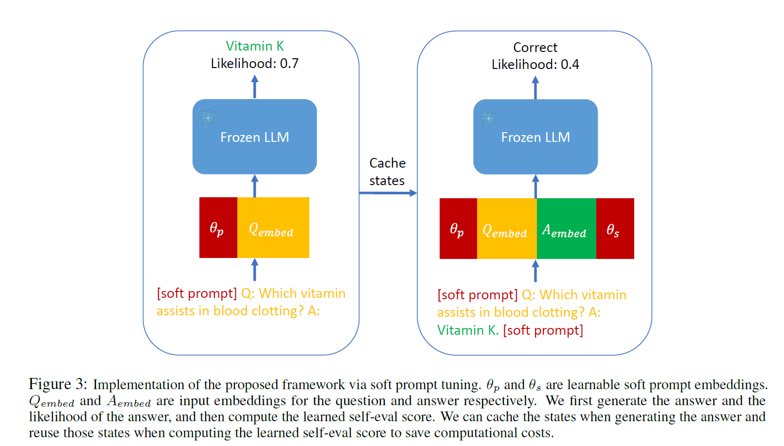
Soft Prompt Tuning

• given query $\mathbf{x} = (x_1, ..., x_{m_q})$
• get embedding of $\mathbf{x}$ to form a matrix $X \in \mathbb{R}^{m_q \times d_e}$
• soft-prompts $\tilde{\theta} \in \mathbb{R}^{l \times d_e}$
• concatenate soft-prompts to query to form $[\tilde{\theta}; X] \in \mathbb{R}^{(m_q + l) \times d_e}$

Adapt to ASPIRE

• update $\theta_p$ with
  $\min_{\theta_p} \mathbb{E}_{(\mathbf{x}, \mathbf{y}) \sim \mathcal{D}^{tr}} {1 \over |\mathbf{y}|} \sum _{j=1} ^{|\mathbf{y}|} - \log f(y_j \ | \ [\theta_p ; X ; Y_{[j-1 ]}])$
• update $\theta_s$ with
  $\min_{\theta_s} \mathbb{E}_{(\mathbf{x}, \mathbf{y}) \sim \mathcal{D}^{tr}} \ \mathcal{L}_c + \mathcal{L}_w \\ \mathcal{L}_c = \mathbb{E}_{\hat{\mathbf{y}} \sim S_c(\mathbf{x}, \mathbf{y})} - \log f(\text{``correct''} \ | \ [\theta_p; X; \hat{Y}; \theta_s]) \\ \mathcal{L}_w = \mathbb{E}_{\hat{\mathbf{y}} \sim S_w(\mathbf{x}, \mathbf{y})} - \log f(\text{``wrong''} \ | \ [\theta_p; X; \hat{Y}; \theta_s]) \\$
• The Inference objective becomes
  $\hat{\mathbf{y}}^* = \argmax_{\hat{\mathbf{y}}} \log f(\hat{\mathbf{y}} \ | \ \mathbf{x};[\theta_p; X])$
• The self-eval score becomes
  $P(\text{correct} \ | \ \mathbf{x}, \hat{\mathbf{y}}^*) = {\exp (\bar{f}(\text{correct} \ | \ [\theta_p; X; \hat{Y}^*; \theta_s]) \over \sum_{z \in \{\text{correct}, \text{wrong} \}} \exp (\bar{f}(z \ | \ [\theta_p; X; \hat{Y}^*; \theta_s])}$

Generation Pipeline

• obtain generated output and the likelihood for the output
• obtain self-eval score
• cache the states of first stage to reduce computational cost for second stage

Computational Complexity

• At test time : $O(l_{max})$
• Predictive entropy and semantic entropy methods : $O(m \cdot l_{max})$

6. Experiments

• Use decoding algorithms that can sample different high-likelihood samples is important
• more training samples lead to enhanced performance
• 2k samples are enough to outperform the baselines without soft-prompt tuning

6.1 Setup

• free-form QA task : CoQA(zero-shot), SQuAD(zero-shot), TriviaQA (5-shot)
• used 50K examples subset
• OPT(350M, 1.3B, 2.7B, 30B), GPT-2(M, L, XL)
• pretrained LLM and $\theta_p$ trained model
• beam-search
• selection score $g(\mathbf{x})$ with PPL, Predictive Entropy, Semantic Entropy, Self-eval, P(True)
• Rouge-L as the evaluation metric $M$ with relatively large $\gamma = 0.7$ (accepting wrong answer is more costly)
• Both stage of training $\theta_p$ and $\theta_s$, 10 epochs with AdamW, batch 8, lr 0.01 and cosine lr scheduling
• for ASPIRE,
  • beam search for $\mathcal{A}$
  • $l = 50$
  • $\hat{\gamma} = 0.9$
  • $k=10$
  • $k_c = 2$
  • $k_w = 10$
  • $\alpha=0.25$
    

6.2 Results

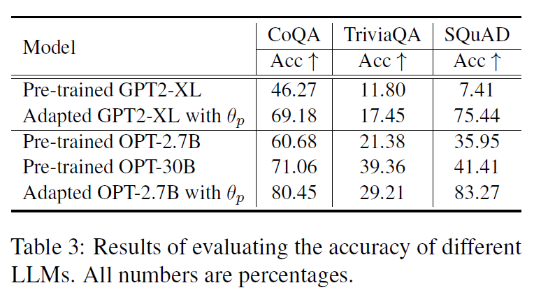
Accuracy

Methods to get selection score

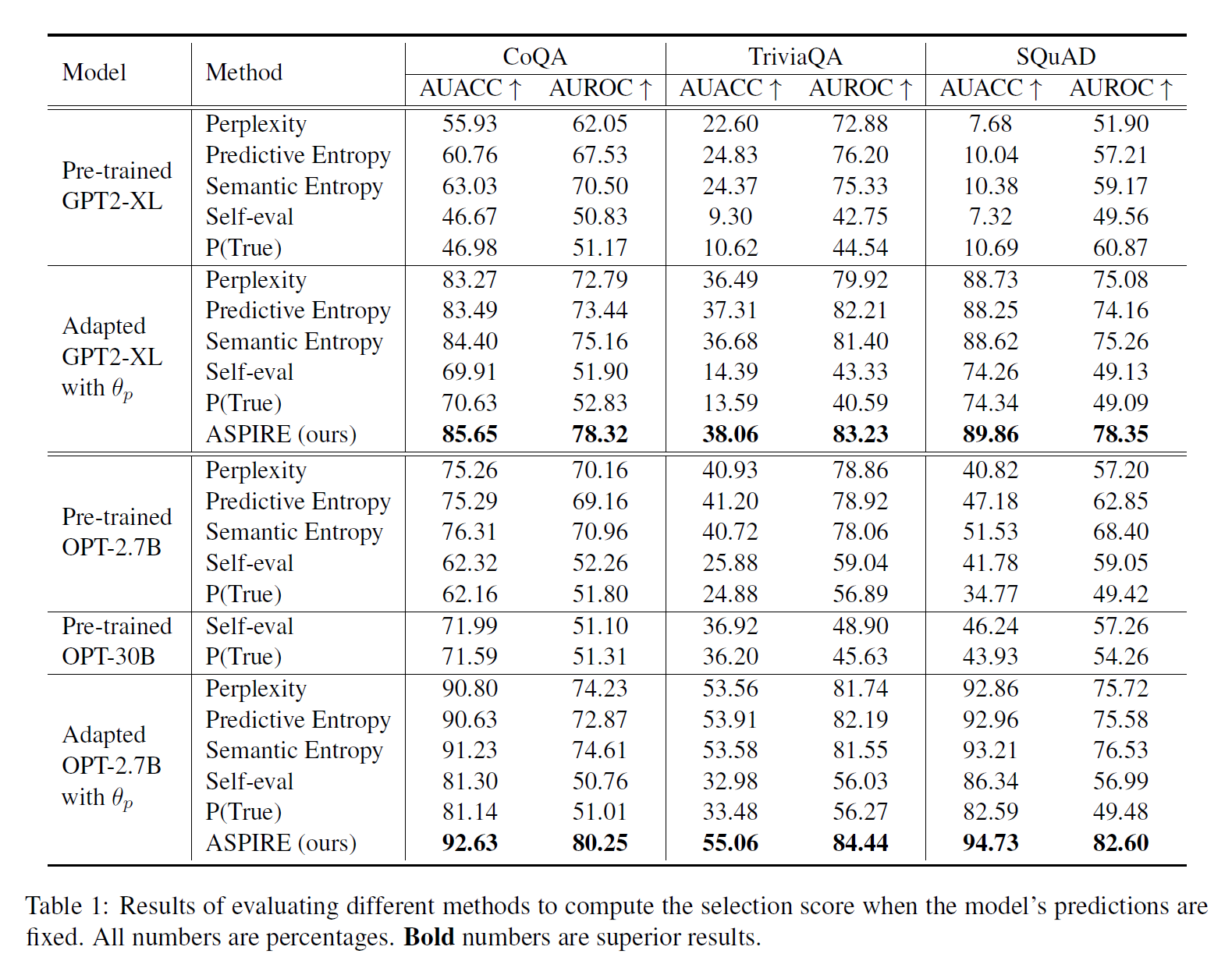
• After prompt tuning, other methods' AUACC is significantly improved as accuracy became better and PPL became more meaningful
• ASPIRE with OPT-2.7B significantly outperforms with Self-eval and P(True) with OPT-30B
• For Self-eval and P(True) method, the AUACC of OPT-30B is better than Adapted OPT-2.7B, it has much worse selective prediction performance
  $\rightarrow$ self-evaluation approach is not effective for high capacity LLMs

6.3 Empirical Analyses

The effect of $\alpha$

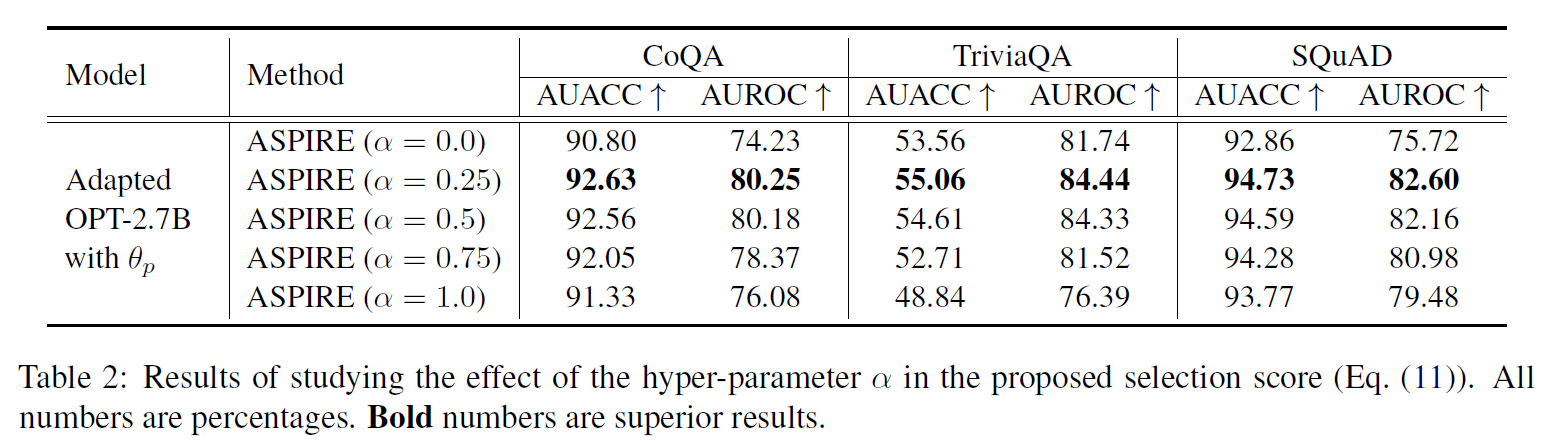
• $\alpha=0.25$ is the best recipe for normalized likelihood and the learned self-eval score
• In practice, this value can be chosen based on the performance on the validation data

The choices of $\mathcal{A}$

• compared beam search and multinomial sampling
• used $k$ highest scoring beams as the answer list (beam search)
• tested temperature 0.1, 1.0, 2.0 for multinomial sampling
  

Training sample efficienty

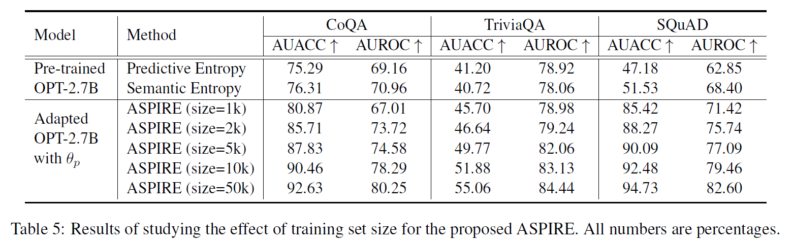
• Fixed the number of steps to be 50K
• ASPIRE can significantly improve selective prediction performance even with limited number of training samples

7. Conclusion

• Adaptation with self-evaluation to improve selective prediction in LLMs
• Soft prompt tuning
• Implement via other PEFT approaches and adapt to larger LLMs (Future work)
• Didn't tested with larger and stringest LLMs (computational constraints)

8. Comment

단순히 프롬프트로 신뢰도를 찍어내는 것이 아니라, 나름의 계산과 Learning 기반으로 신뢰도를 얻어낼 수 있는게 좋았음. 다만 테스트한 모델이 좀 오래되어서, 최근의 sLLM으로도 가능한지 의문