1. Introduction

LLM Hosting

• High inference cost
• High energy consumption

As model size grows, the memory bandwidth becomes a major bottleneck.
When deploying these models on distributed systems or multi-device platforms, the inter-device communication overhead impact the inference latency and energy consumption.
$\Rightarrow$ Quantization

Most existing quantization $\rightarrow$ post-training

• simple and easy to apply
• significant loss of accuracy when precision goes lower (not optimized for quantized representation)

Quantization-aware training

• better accuracy
• continue-train or fine-tuning
• hard to converge when precision goes lower
• unknown whether it follows the scaling law of LMs

Previous Trial

• CNN
• BERT machine translation

BitNet

• 1-bit transformer architecture
• scale efficiently in terms of both memory and computation
• binary weights + quantized activations
• high precision for optimizer states and gradients
• simple implementation
• complements other acceleration methods (PagedAttention, FlashAttention, speculative decoding)
• Compared with FP16 Transformers (PPL, downstream task)
• follows a scaling law of full-precision transformer

2. BitNet

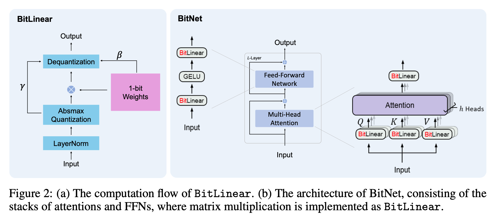
• BitLinear instead of matrix multiplication
• other components are left as 8-bit precision
  • residual connection and LayerNorm have negligible computation costs
  • QKV transformation cost is also much smaller than the parametric projection
  • models have to use high-precision probabilities to perform sampling (leave input/output embedding as high precision)

2.1 BitLinear

1. Binarize weights to +1 or -1 with signum function

• Centralize to be zero-mean to increase the capacity witnin a limited numerical range
• Use scaling factor $\beta$ after binarization to reduce l2 error between real-valued and the binarized.

2. Quantize activations to $b$-bit precision with absmax

• $Q_b = 2^{b-1}$

• $\epsilon$ is a small floating-point number that prevents overflow in clipping

  $\tilde{x} = \text{Quant}(x) = \text{Clip} \left( x \times {Q_b \over \gamma}, -Q_b + \epsilon , Q_b - \epsilon \right)$
  $\gamma = ||x||_{\infin}$

• For activations before non-linear functions (ReLU) $\rightarrow$ scale into $[0, Q_b]$ by subtracting the minimum of the inputs

  $\tilde{x} = \text{Quant}(x) = \text{Clip} \left( (x-\eta) \times {Q_b \over \gamma}, \epsilon, Q_b - \epsilon\right)$
  $\eta = \min _{ij} x_{ij}$

• quantize with 8-bit

• Training $\rightarrow$ quantize per tensor / Inference $\rightarrow$ quantize per token

3. Matrix Multiplication
   $y = \tilde{W} \tilde{x}$

The variance of the output $y$ under following assumption

• the elements in $W$ and $x$ are mutually independent and share same distribution
• $W$ and $x$ are independent of each other

In full-precision, $\text{Var}(y) = 1$ with standard initialization method $\rightarrow$ training stability. To preserve this stability, use LayerNorm function.

• $\text{Var}(y) \approx E[\text{LN}(\tilde{x})^2] = 1 \quad \quad \quad (\text{SubLN})$

Then, the final representation of BitLinear is:

${\beta\gamma \over Q_b}$ means Dequantization to restore original precision

4. Model Parallelism with Group quantization and Normalization

• Calculate all parameters $\alpha, \beta, \gamma, \eta$ with each group (device)
• If the Number of group is $G$, then the parameter becomes
  $\alpha_g = {G \over nm} \sum _{ij} W_{ij} ^{(g)}, \quad \quad \beta_g = {G \over nm} ||W^{(g)}||_1, \\ \gamma_g = ||x^{(g)}||_{\infin}, \quad \quad \eta_g = \min _{ij} x_{ij} ^{(g)}$
• LayerNorm should also be applied with similar way

2.2 Model Training

Straight-through estimator

• ignore non-differentiable functions (Clip, Sign) during backpropagation

Mixed Precision training

• weights and activations $\rightarrow$ low precision
• gradients and optimizer states $\rightarrow$ high precision
• latent weight $\rightarrow$ high precision (binarized on the fly during forward pass and never used for the inference process)

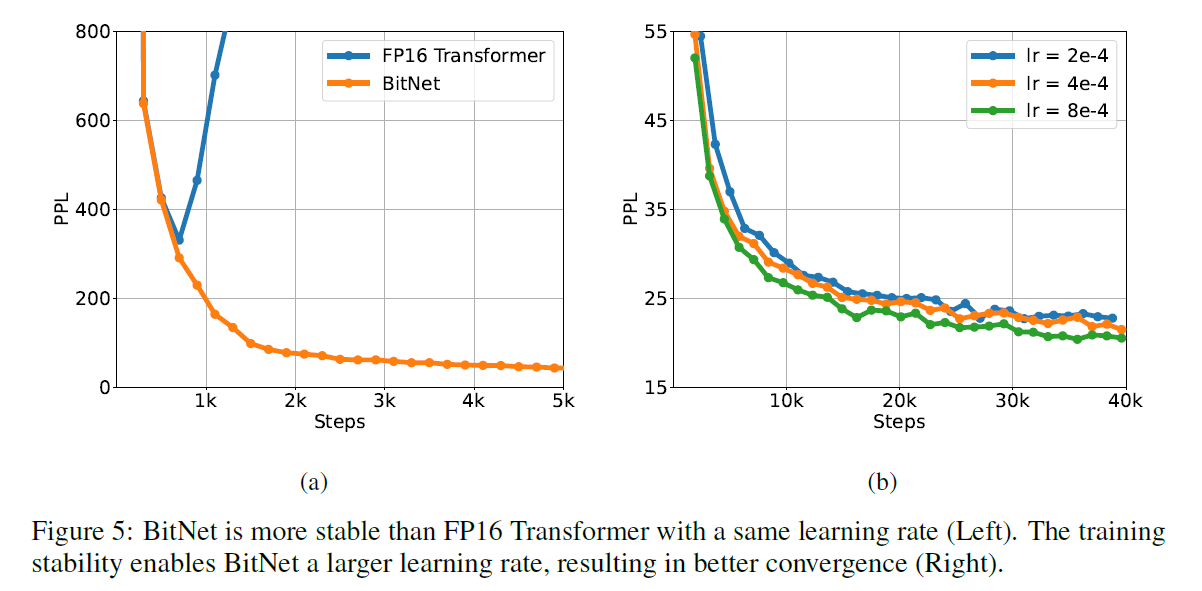
Large Learning Rate

• Small update on latent weight makes no difference in the 1-bit weights
• even worse at the beginning of training
• BitNet benefits from this method whild FP16 Transformer diverges at the beginning of training

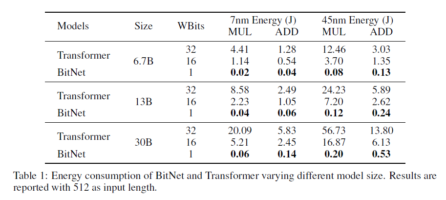
2.3 Computational Efficiency

Arithmetic Operations

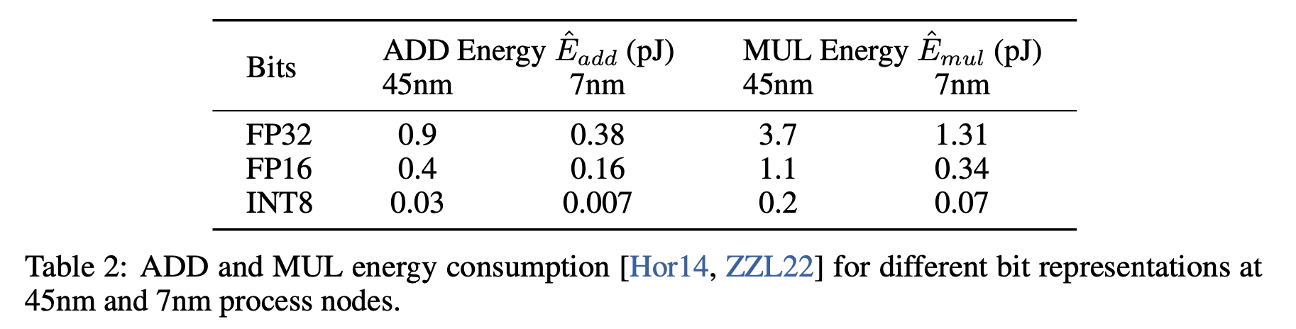
Energy Consumption during matrix multiplication

Multiplying $m \times n$ and $n \times p$ matrices

• Vanila Transformer

  $\begin{aligned} E_{add} &= m \times (n-1) \times p \times \hat{E}_{add} \\ E_{mul} &= m \times n \times p \times \hat{E}_{mul} \end{aligned}$

• BitNet $\rightarrow$ multiplication is dominated by the addition as weights is 1-bit

  $E_{mul} = (m \times p \ + m \times n) \times \hat{E}_{mul}$

  

3. Comparision with FP16 Transformers

3.1 Setup

• 125M to 30B model
• Sentencepiece with vocab 16K
• Pile, Common Crawl, RealNews, CC-Stories dataset
• Transformer baseline

3.2 Inference-Optimal Scaling Law

The loss scales as the power law with the amount of computation

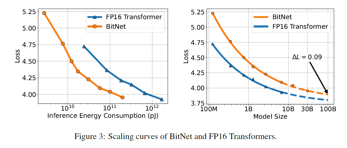
• Loss gap between FP16 and BitNet gets lower
• It doesn't properly model the relationship between the loss and the actual compute
• calculating FLOP doesn't work as the weight is 1-bit
• mainly measures the training computation

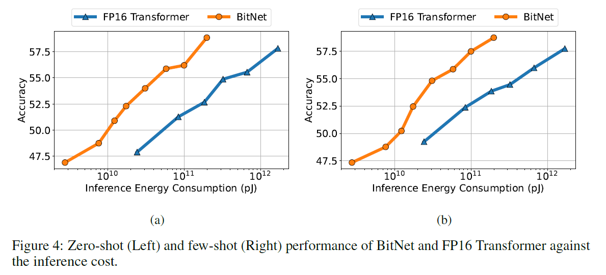
Inference-Optimal Scaline Law

• Loss against Energy Consumption
• inference energy cost
• Significantly better loss and inference cost is much smaller

3.3 Downstream Task

0-shot and 4-shot result

3.4 Stability Test

Varying peak Learning Rates

4. Comparison with Post-training Quantization

4.1 Setup

• Transformer (W16A16)
• SmoothQuant(W4A4)
• GPTQ (W2A16)
• BitNet(W1A8)
• QuIP(W2A16)

4.2 Result

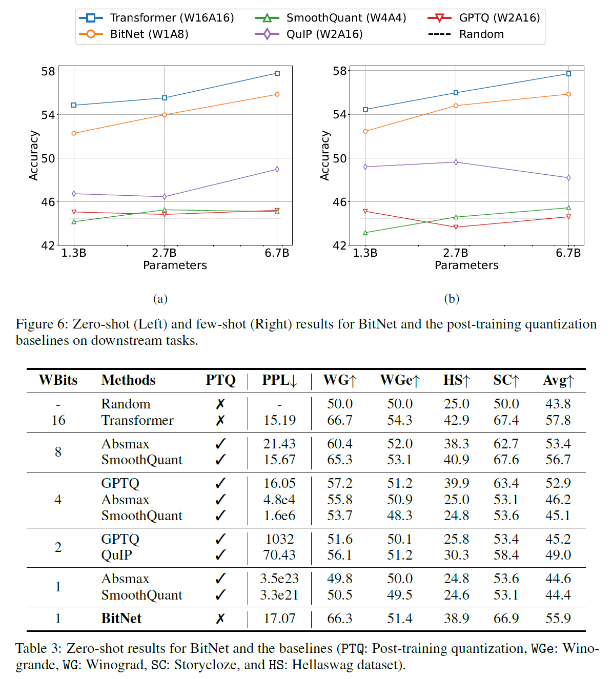
• In 4-bit Models, weight-only quantization methods outperform the weight-and-activation quantizers as activation is harder to quantize
• In Low-Bit model, significantly achieves better results than other models
• BitNet has consistently superior scores over all baselines (Quantization-Aware Training > Post training quantization)

5. Ablation studies

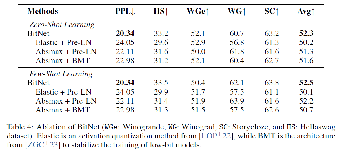
• Quantization method : Absmax, Elastic function
• LayerNorm : SubLM, Pre-LN, BMT

6. Conslusion

• 1-bit Transformer
• scalable and stable
• Performance on PPL and Downstream task
• reducing memory footprint, energy consumption
• Scaling Law