1. Introduction

• Unsupervised Language Models $\rightarrow$ trained on data generated by humans.
• It cannot understand common mistakes by human (human want the model to be biased to high-quality answer)
• It is important to select the model's desired responses and behavior from its knowledge. $\rightarrow$ Using RL
• Existing skills $\rightarrow$ using curated sets of human preference
  (pretraining $\rightarrow$ preference learning)
• But the most efficient strategy is SFT

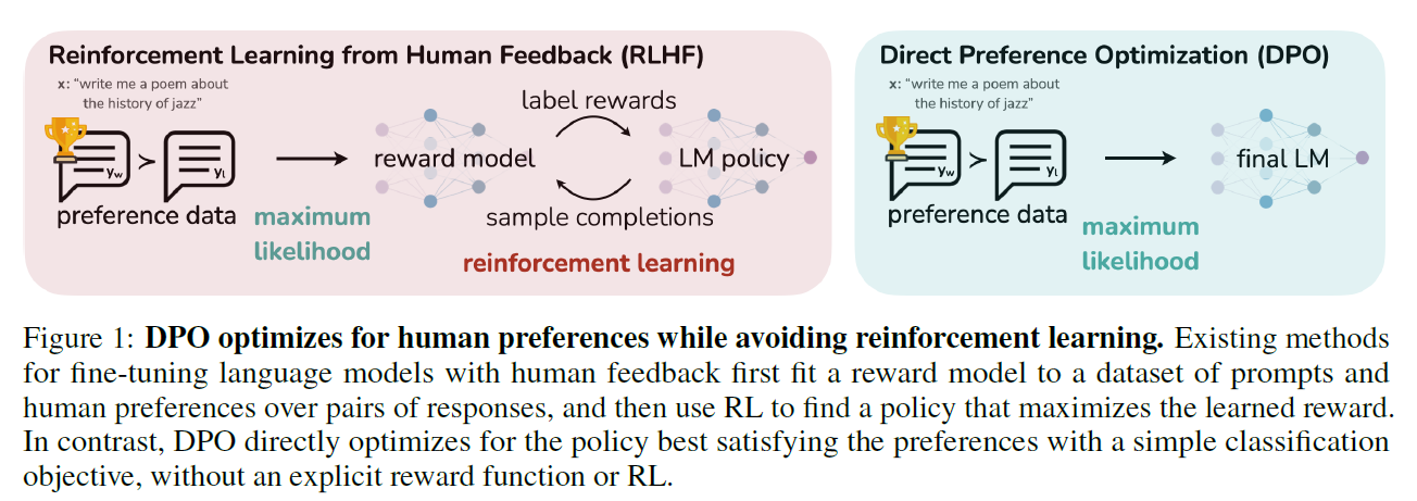
RLHF

• Fit a reward model to a human preference
• After that, use RL to optimize a language model policy
• more complex than SFT (training multiple LMs, sampling from the LM policy)

DPO (Direct Preference Optimization)

• Without explicit reward modeling / RL
• implicitly optimizes the same objective as existing RLHF (reward maximization with KL-divergence constraint)
• simple to implement, starightforward to train
• dynamic, per-example importance weight $\rightarrow$ prevents model degeneration
• rely on theoretical preference model (Bradley-Terry / Plackett-Luce)
• define the preference loss as a function of the policy
  

2. Related Work

• Zero-Shot, Few-Shot
• instruction tuning
• fine-tune on human preference datasets under BT, PL model (RLHF, using PPO, REINFORCE)

Outside the context of LM

• Learning Policies from preferences has been studied in both bandit and reinforcement learning settings.
• Contextual Bandit Learning (CDB, Contextual Dueling Bandit, using Von Neumann Winner(policy whose expected win rate against any other policy is at least 50%))
• Preference-Based RL (learning binary preference generated by unknown scoring function)

3. Preliminary

Review RLHF Pipelines

SFT Phase

• Fine Tune LM with high-quality dataset of downstream task
• Obtain $\pi^{\text{SFT}}$

Reward Modeling Phase

• Use SFT Model $\pi^{\text{SFT}}$ and prompt $x$ to get pairs of answers $y_1$ and $y_2$

  • $(y_1, y_2) \sim \pi^{\text{SFT}} (y \ | \ x)$

• Human labels the answer

  • $y_w \succ y_l$ (winner and loser)

• These are assumed to be generated by some latent reward model $r^* (y, x)$

  • Actually this is not accessable
  • use Bradley-Terry or Plackett-Luce

• BT model's human preference distribution $p^*$

  • $\begin{aligned} p^*(y_1 \succ y_2 | x) &= {{\exp (r^* (x, y_1))} \over {\exp(r^*(x, y_1)) + \exp(r^*(x, y_2))}} \\ &={1 \over 1 + \exp\left( r^*(x, y_2) - r^*(x, y_1)\right)} \\ &= \sigma(r^*(x, y_2) - r^*(x, y_1)) \end{aligned}$

• Assuming a static dataset $\mathcal{D} = \{ x^{(i)}, y_w^{(i)}, y_l^{(i)} \}_{i=1} ^N$ sampled from $p^*$, parametrize a reward model $r_{\phi}(x, y)$ and estimate the parameters using maximum likelihood

  • For Binary Classification, the negative log-likelihood is
    $\mathcal{L}_\text{R} (r_{\phi}, \mathcal{D}) = -\mathbb{E}_{(x, y_w, y_l) \sim \mathcal{D}} [log \ \sigma (r_{\phi} (x, y_w) - r_{\phi} (x, y_l))]$ where $\sigma$ is logistic function
  • for Language Model, $r_{\phi}(x, y)$ is often initialized from $\pi^{\text{SFT}}(y \ | \ x)$ with the addition of a linear layer on top of the final transformer layer $\rightarrow$ produces a single scalar prediction

RL Fine-Tuning Phase

• Use learned reward function to provide feedback to the language model

  • the optimizing problem is formulated as
    $\max_{\pi_\theta} {\mathbb{E}_{x \sim \mathcal{D}, y \sim \pi_\theta (y \ | \ x)} [r_{\phi} (x,y)] - \beta \mathbb{D}_{\text{KL}} [\pi_\theta (y \ | \ x) \ || \ \pi_{\text{ref}} (y \ | \ x)]}$
  • $\beta$ is a parameter controlling the deviation from the base reference policy $\pi_{\text{ref}}$ (namely, $\pi^{\text{SFT}}$)
  • In practice, $\pi_\theta$ is also initialized to $\pi^{\text{SFT}}$
  • As language generation is descrete, use reward function
    $r(x,y) = r_{\phi}(x,y) - \beta(\log \pi_\theta (y \ | \ x) - \log \pi_{\text{ref}}(y \ | \ x))$ and maximize with PPO

Bradley-Terry Model (for backup)

Rank entities by pairwise comparisons

where $p$ is real-valued score

Plackett-Luce Model (for backup)

Rank entities by its worth

4. Direct Preference Optimization

• Applying RL to large-scale model is challenging
• DPO bypasses the reward modeling step and directly optimizes a LM using preference data

Deriving DPO Objective

Start with RL objective as prior work

the optimal solution is

Even if we use MLE estimate $r_{\phi}$ of the ground-truth reward function $r^*$, it is difficult to estimate $Z(x)$ which is the partition function.
Using Logarithm, the reward function is expressed as

For Bradley-Terry case, using $r(x,y)$ above, the optimal RLHF policy $\pi^*$ satisfies

Then the DPO loss becomes

Finally, the loss is independent of $r$ which means it bypasses the explicit reward modeling step. Also, the theoretical property of Bradley-Terry model holds.

What does the DPO update to?

The gradient of the Loss function of DPO with respect to $\theta$ is

where $\hat{r_\theta} (x,y) = \beta \log {\pi_\theta (y \ | \ x) \over \pi_{\text{ref}} (y \ | \ x)}$ is the reward implicitly defined by two LMs.

This loss increases the likelihood of $y_w$ and decreases the likelihood of $y_l$. Also, the examples are weighed by how much $\hat{r_\theta} (x,y)$ dispreferred $y_l$, scaled by $\beta$.
Our experiment suggests the importance of weighing.

DPO outline

The general DPO pipeline is:

• Sample completions $y_1$, $y_2$ from reference model $\pi_{\text{ref}}$

• label with human preference to construct offline dataset $\mathcal{D} = \{x^{(i)}, y_w^{(i)}, y_l^{(i)} \}$

• Optimize the language model $\pi_\theta$ to minimize $\mathcal{L}_{\text{DPO}}$ given $\pi_{\text{ref}}$ and $\mathcal{D}$ and $\beta$ (Also one can reuse publicly available dataset)

• If $\pi^{\text{SFT}}$ is available, set $\pi_{\text{ref}} = \pi^{\text{SFT}}$ otherwise, set $\pi_{\text{ref}}$ by maximizing likelihood of preferred completions $(x, y_w)$

  5. Theoretical Analysis of DPO

  5.1 Your Language Model Is Secretly a Reward Model

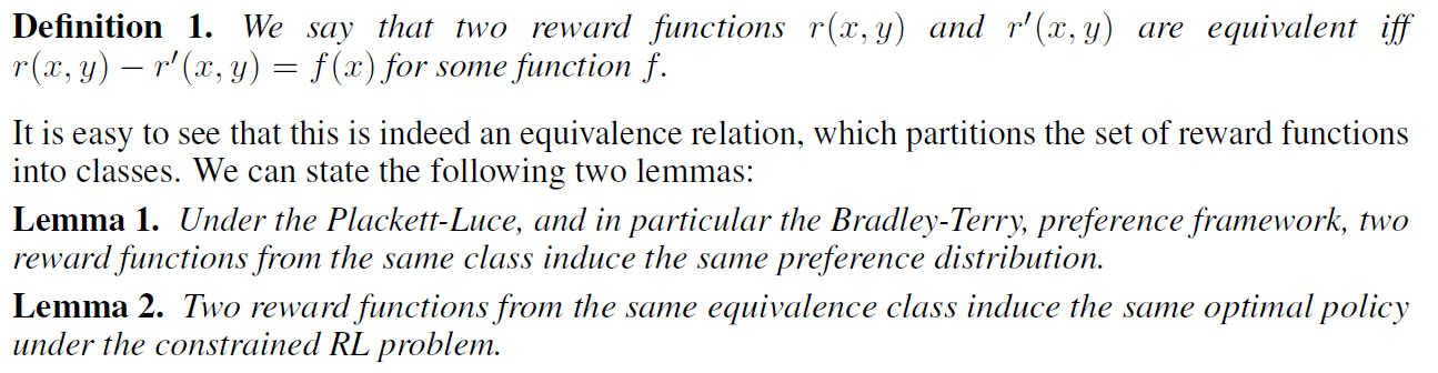
First Lemma is well-known under-specification issue with Plackett-Luce family. We should impose additional idenfifiability constraints. The final objective is to recover an arbitrary reward function from the optimal class.

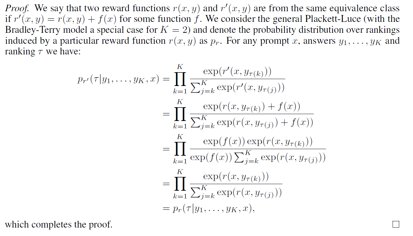
Proof for Lemma 1

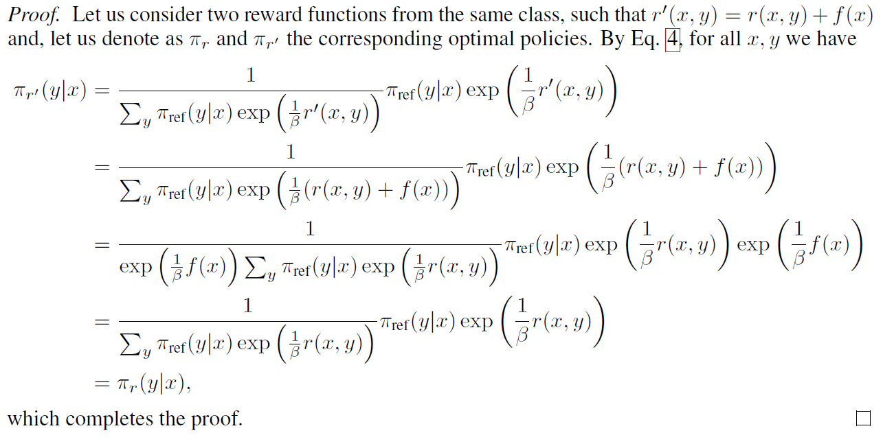
Proof for Lemma 2

Theorem 1 also specifies exactly which reward function within each equivalence class the DPO reparameterization selects.
The reward function satisfies

i.e. $\pi(y \ | \ x)$ is valid distribution.
Also, we can impose certain constraints on the under-constrained Plackett-Luce family such that we preserve the class of reward models.

5.2 Instability of Actor-Critic Algorithms

In RL Fine-Tuning step from RLHF, the optimization objective is

This is equivalent reward to DPO. Without the normalization term in $f$ which can be interpreted as the soft value function of $\pi_{\text{ref}}$, the learning could be unstable as the policy gradient could have high variance.
Prior work used human completion based reward normalization but DPO yields baseline-free reward.

6. Experiments

• well-controlled text-generation : maximize reward and minimize KL-divergence

  • IMDb
  • preference pair : pretrained sentiment classifier
  • SFT : GPT-2-large

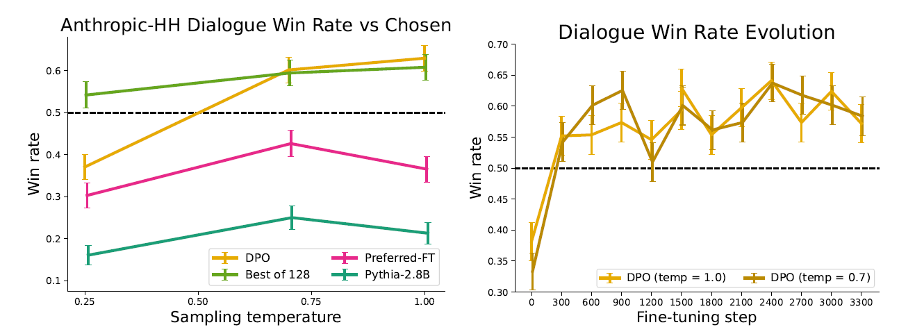
• summarization and dialog : DPO performance on larger models and more difficult RLHF task

  • Summarization : Reddit TL;DR dataset
  • Single-Turn dialogue : Anthropic Helpful and Harmless dataset

• Evaluation with win rate against baseline policy, GPT-4 for proxy of human
  
  
  
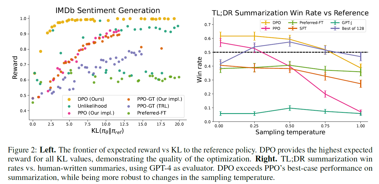
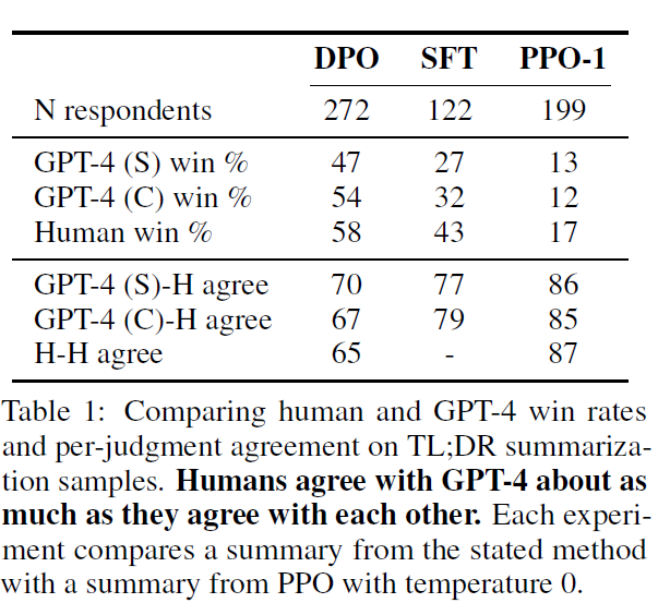
  GPT-4(S) : "Which Summary is better?"
  GPT-4(C) : "Which Sumary is more concise?"

7. Discussion

• rather than standard RL approach, DPO identifies a mapping between LM policies and reward functions
  $\rightarrow$ training LM to satisfy human preference directly with simple cross entropy loss without RL
• No hyperparameter tuning is enough to perform like RLHF
• Need High-Quality Automated Judgement (GPT-4 is impacted by prompt)
• This study applied DPO up to 6B models $\rightarrow$ larger models?