Is Cosine-Similarity of Embeddings Really About Similarity?

임재석·2024년 3월 15일

Embedding

paper-study

목록 보기

13/23

1. Introduction

Discrete Entities are embedded to dense real-valued vectors
- word embedding for LLM
- recommender system
The embedding vector can be used as input to other models
Also, they can provide a data-driven notion of similarity between entities
Cosine Similarity has become a very popular measure of semantic similarity
- the norm of the embedding vectors is not as important as the directional alignment between the embedding vectors
- unnormalized dot-product is not worked
Cosine similarity of the learned embeddings can in fact yield arbitrary results
- learned embeddings have a DoF that can render arbitrary cosine-similarities even though their dot-products are well-defined and unique
propose linear Matrix Factorization models as analytical solutions

2. Matrix Factorization Models

focus on linear models as they follow for closed-form solutions
matrix $X \in \mathbb{R}^{n \times p}$ , conatining $n$ data points and $p$ features
the goal is to estimate a low-rank matrix $AB^{\top} \in \Reals ^{p \times p}$ where $A, B \in \Reals^{p \times k}$ with $k \le p$ such that $XAB^{\top}$ is a good approximation of $X \approx XAB^{\top}$
$X$ is a user-item matrix
- the row $\vec{b_i}$ of $B$ : item-embeddings ( $k$ -dimensional)
- the row $\vec{x_u} \cdot A$ of $XA$ : user-embeddings
- the embedding of user $u$ is the sum of the item-embeddings $\vec{a_j}$ that the user has consumed
this is defined in terms of the unnormalized dot-product between two embeddings
- $(XAB^{\top})_{u,i} = \lang \vec{x_u} \cdot A, \vec{b_i} \rang$
- once it has been learned, it is common to consider
  - two items cosine similarity
  - two users cosine similarity
  - user-item cosine similarity
- this can lead to arbitrary results and they may not even be unique

2.1 Training

the key factor affecting the utility of cosine similarity is the regularization employed when learning the embeddings in $A, B$
- $\min_{A, B} || X - XAB^{\top} || _F ^2 + \lambda ||AB^{\top}||_F^2$
- $\min_{A, B} || X - XAB^{\top} || _F ^2 + \lambda (||XA||_F^2 + ||B||_F^2)$
First one applies $||AB^{\top}||_F^2$ to their product
- in Linear models, this L2-regularization is equivalent to learning with denoising (drop-out in the input layer)
- the resulting prediction accuracy os test data was superior to the second objective
- denoising/drop-out is better than weight decay (second one)
Second one is equivalent to the usual matrix factorization objective
- $|| X - PQ^{\top} || _F ^2 + \lambda (||P||_F^2 + ||Q||_F^2)$
- regularizing $P$ and $Q$ separately is similar to weight decay in deep learning
if $\hat{A}, \hat{B}$ are solutions of objective, for an arbitrary rotation matrix $R \in \Reals^{k \times k}$ are the solutions as well
cosine similarity is invariant under rotation $R$
only the first objetive is invariant to rescalings of the columns of $A$ and $B$ (different latent dimensions of the embeddings)
- if $\hat{A}\hat{B}^{\top}$ is the solution of the first objective, for an arbitrary diagonal matrix $D \in \Reals^{k \times k}$ , $\hat{A}DD^{-1}\hat{B}^{\top}$ is the solution also
- Then devine a new solution as a function of $D$ as
  $\begin{aligned} \hat{A}^{(D)} &:= \hat{A}D \\ \hat{B}^{(D)} &:= \hat{B}D^{-1} \end{aligned}$
- this diagonal matrix $D$ affects the normalization of the learned user and item embeddings (rows)
  $\begin{aligned} (X\hat{A}^{(D)})_{(\text{normalized})} &= \Omega_A X\hat{A}^{(D)} = \Omega_A X\hat{A}D \\ \hat{B}^{(D)}_{\text{(normalized)}} &= \Omega_B \hat{B}^{(D)} = \Omega_B \hat{B}D^{-1} \end{aligned}$
  where $\Omega$ is appropriate diagonal matrices to normalize each learned embedding to unit Euclidian norm
- a different choice for $D$ cannot be compensated by the $\Omega$
- they depend on $D$ so they can be shown as $\Omega_A(D), \Omega_B(D)$
- cosing similarities of the embeddings depend on this arbitrary matrix $D$
the cosine similarity becomes
- item - item $\text{cosSim}(\hat{B}^{(D)}, \hat{B}^{(D)}) = \Omega_B(D) \cdot \hat{B} \cdot D^{-2} \cdot \hat{B}^{\top} \cdot \Omega_B(D)$
- user-user $\text{cosSim}(X\hat{A}^{(D)}, X\hat{A}^{(D)}) = \Omega_A(D) \cdot X\hat{A} \cdot D^{2} \cdot (X\hat{A})^{\top} \cdot \Omega_A(D)$
- user-item $\text{cosSim}(X\hat{A}^{(D)}, \hat{B}^{(D)}) = \Omega_A(D) \cdot X\hat{A} \cdot \hat{B}^{\top} \cdot \Omega_B(D)$
These cosine similarities all depend on arbitrary matrix $D$
user-user and item-item is directly depend on $D$ while user-item is indirectly depend on $D$ due to its effect to normalizing matrices

2.2 Details on First Objective

The closed-form solution of the first objective is $\hat{A}_{(1)}\hat{B}_{(1)} = V_k \cdot \text{dMat}(..., {1 \over 1 + \lambda/\sigma_i^2}, ...)_k \cdot V_k^{\top}, \quad X =: U\Sigma V^{\top}, \quad \Sigma = \text{dMat}(..., \sigma_i, ...)$ and $V_k$ is truncated matrices of rank $k$
Sine $D$ is arbitrary, w.l.o.g. we may define $\hat{A}_{(1)} = \hat{B}_{(1)} := V_k \cdot \text{dMat}(..., {1 \over 1 + \lambda/\sigma_i^2}, ...)_k^{{1 \over 2}}$
when we think of the special case of a full-rank MF model, this would be two cases
- choose $D = \text{dMat}(..., {1 \over 1 + \lambda/\sigma_i^2}, ...)^{{1 \over 2}}$
  - $A_{(1)}^{(D)} = \hat{A}_{(1)} \cdot D = V \cdot \text{dMat}(..., {1 \over 1 + \lambda/\sigma_i^2}, ...)$
  - $B_{(1)}^{(D)} = \hat{B}_{(1)} \cdot D^{-1} = V$
  - given the matrix of normalized singular vectors $V$ , the normalization $\Omega_B = I$
  - Then $\text{cosSim}(\hat{B}_{(1)}^{(D)}, \hat{B}_{(1)}^{(D)}) = VV^{\top} = I$
  - Cosine similarity between any pair of item-embedding is zero
  - $\text{cosSim}(X\hat{A}_{(1)}^{(D)}, \hat{B}_{(1)}^{(D)}) = \Omega_A \cdot X \cdot V \cdot \text{dMat}(..., {1 \over 1 + \lambda/\sigma_i^2}, ...) \cdot V^{\top} = \Omega_A \cdot X \cdot \hat{A}_{(1)}\hat{B}_{(1)}^{\top}$
  - the only difference in user-item embeddings is the normalization $\rightarrow$ the same ranking ( $\Omega_A$ is irrelevant)
- choose $D = \text{dMat}(..., {1 \over 1 + \lambda/\sigma_i^2}, ...)^{-{1 \over 2}}$
  - similar to previous case
  - $A_{(1)}^{(D)} = \hat{A}_{(1)} \cdot D^{-1} = V$
  - $B_{(1)}^{(D)} = \hat{B}_{(1)} \cdot D = V \cdot \text{dMat}(..., {1 \over 1 + \lambda/\sigma_i^2}, ...)$
  - $\text{cosSim}(X\hat{A}_{(1)}^{(D)}, X\hat{A}_{(1)}^{(D)}) = \Omega_A \cdot X \cdot X^{\top} \cdot \Omega_A$
  - for user-user similarities, it is based on the raw data-matrix
  - it doesn't uses the learned embeddings
  - $\text{cosSim}(X\hat{A}_{(1)}^{(D)}, \hat{B}_{(1)}^{(D)}) = \Omega_A \cdot X \cdot \hat{A}_{(1)} \cdot \hat{B}_{(1)}^{\top} \cdot \Omega_B$
  - $\Omega_B$ normalizes the rows of $B$ but this is again the same rankings
  - $\text{cosSim}(\hat{B}_{(1)}^{(D)}, \hat{B}_{(1)}^{(D)}) = \Omega_B \cdot V \cdot \text{dMat}(..., {1 \over 1 + \lambda/\sigma_i^2}, ...)^{2} \cdot V_{\top} \cdot \Omega_B$
  - this is very different from the previous choice
- Hence, the different choice of $D$ result in different cosine-similarities even though the learned model $\hat{A}_{(1)}^{(D)}\hat{B}_{(1)}^{(D)\top} = \hat{A}_{(1)}\hat{B}_{(1)}^{\top}$ is invariant to $D$
- the results of cosine-similarity are arbitrary and not unique for this model

2.3 Details on Second Objective

The solution of the second objective is
- $\hat{A}_{(2)} = V_k \cdot \text{dMat}(..., \sqrt{{1 \over \sigma_i} \cdot (1 - {\lambda \over \sigma_i})_+}, ...)_k$
- $\hat{B}_{(2)} = V_k \cdot \text{dMat}(..., \sqrt{\sigma_i \cdot (1 - {\lambda \over \sigma_i})_+}, ...)_k$
- $(y)_+ = \max(0, y)$
If we use usual notation of MF $P = XA$ and $Q = B$ ,
- we get $\hat{P} = X\hat{A}_{(2)} = U_k \cdot \text{dMat}(..., \sqrt{{1 \over \sigma_i} \cdot (1 - {\lambda \over \sigma_i})_+}, ...)_k$
- this diagonal matrix is same for user and item embeddings due to its symmetry in the L2-norm regularization
- this solution is unique $\rightarrow$ there is no way to choose arbitrary matrix $D$
In this case, the cosine-similarity yields unique results
is this matrix $\text{dMat}(..., \sqrt{{1 \over \sigma_i} \cdot (1 - {\lambda \over \sigma_i})_+}, ...)_k$ the best possible semantic similarities?
- comparing this case with 2.2 gives the arbitrary diagonal matrix $D$ in 2.2 may be chosen as $D = \text{dMat}(..., \sqrt{{1 \over \sigma_i}}, ...)_k$

3. Remedies and Alternatives to Cosine-Similarity

when a model is trained w.r.t. the dot-product, its effect on cosine-similarity can be opaque and sometimes not even unique
- train model on cosine-similarity $\rightarrow$ use layer normalization
- project the embedding back into the original space $\rightarrow$ cosine-similarity works
  - view $X\hat{A}\hat{B}^{\top}$ as the raw data's smoothed version and the rows of $X\hat{A}\hat{B}^{\top}$ as the users' embeddings in the original space
in cosine-similarity, normalization is applied after the embeddings have been learned
- this can reduce the result similarities compare to applying some normalization or reduction of popularity bias before of during learning
To resolve this,
- standardize data $X$ (zero mean, unit variance)
- negative sampling, inverse propensity scaling to account for the different item popularities
  - word2vec is trained by sampling negatives with a probability proportional to their frequency

4. Experiments

illustrate these findings for low-rank embeddings
Not aware of a good metric for semantic similarity $\rightarrow$ experiments on simulated data $\rightarrow$ ground-truths are known (clustered items data)
generated interactions between 20000 users and 1000 items assigned to 5 clusters with probability $p_c$
sampled the powerlaw-exponent for each cluster $c$ , $\beta_c \sim \text{Uniform}(\beta_{min}^{(item)}, \beta_{min}^{(item)})$
- where $\beta_{min}^{(item)} = 0.25, \beta_{min}^{(item)} = 1.5$
assigned a baseline popularity to each item $i$ according to the powerlaw $p_i = \text{PowerLaw}(\beta_c)$
then generated the items that each user $u$ had interacted with
- firstly, randomly sampled user-cluster preferences $p_{uc}$
- compute the user-item probabilities $p_{ui} = {p_{uc_i}p_i \over \sum _i p_{uc_i}p_i}$
- sampled the number of items for this user $k_u \sim \text{PowerLaw}(\beta^{(user)})$ (used $\beta^{(user)} = 0.5$ and sampled $k_u$ items with $p_{ui}$ )
Learned the matrices $A, B$ with two training objective ( $\lambda = 10000$ and $\lambda = 100$ )
- low-rank constraint $k=50$ , $p=1000$ to complement the analytical result for the full-rank case above

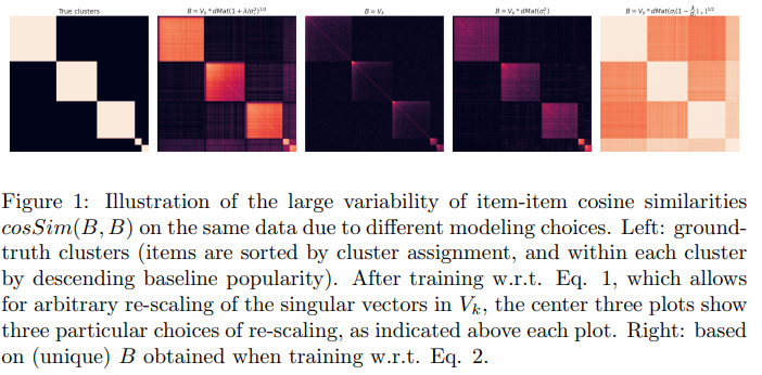
Left one is ground-truth item-item similarities
training with first objective and chose three re-scaling of the singular vectors in $V_k$ (middle three)
Right one is trained with second objective $\rightarrow$ unique solution
see how vastly different the resulting cosine-similarities can be even for reasonable choice of re-scaling (not used extreme case)

5. Conclusions

cosine similarities are heavily dependent on the method and regularization technique
in some cases, it can be rendered even meaningless
cosine-similarity with the embeddings in deep models to be plagued by similar problems
- deep model's different layers may be subject to different regularization $\rightarrow$ may affect $D$