1. Introduction

• SOTA models' complexity $\rightarrow$ computation / memory / communication bandwidth
  • LoRA
  • quantizing model parametros
• Prior work has been limited to fine-tuning $\rightarrow$ tools for pretrain from scratch is absent

Can neural networks be trained from scratch using Low-Rank Adapters?

• common computing clusters often have slower cross-node training with gradient accumulation as slow communication speed and bandwidth
  • Low-Rank adapters compress the communication between these processors while preserving essential structural attributes
• Vanila LoRA underperforms in training a model from scratch
  • using parallel low-rank updates can bridge this gap

Difference to existing works

• data and model parallelism

  • stores different copies of the LoRA parameters

  • trained on different shards

    • different from traditional federated learning which replicates the same model across devices

  • their method enables distributed training with infrequent synchronizations allowing for single-device inference

• Previous works
  • ReLoRA : trains and merges LoRA into main weights
  • FedLoRA : train LoRA parameters for finetuning within a federated learning framework $\rightarrow$ training multiple LoRA and averaging them
  • AdaMix : averages all MLP in MoE into a single MLP $\rightarrow$ needs constant synchronization during the forward and backward pass

2. Preliminaries

• $x$ as a scalar, $\mathbf{x}$ as a vector, $X$ as a matrix, $\mathcal{X}$ as a distribution or a set
• $f$ as a function, $F(\cdot)$ as a composition of functions, $\mathcal{L}(\cdot, \cdot)$ as a loss-function

2.1 Parameter Efficient adapters

• Adapters : trainable functions that modify existing layers in an neural network

• LoRA : subclass of linear adapters

  • the linearity of LoRA allows for the trained parameters to be integrated back in to the existing weights
  • the linearity allows models to maintain the original inference cost

LoRA

• Given input $\mathbf{x} \in \reals^n$ and a linear layer $f(\cdot) : \reals^n \rightarrow \reals^m$ parameterized by the weight $W \in \reals^{m \times n}$

• LoRA re-parameterizes the function as

  • $f_{\text{lora}}(x) = \mathbf{W}\mathbf{x} + s \mathbf{BAx}$
  • $\mathbf{B} \in \reals^{m\times r}$, $\mathbf{A} \in \reals^{r \times n}$, $s \in \reals$
  • rank $r << \min(m, n)$

• Forward pass incurs an extra computational overhead

• the significance of LoRA pertains to the optimizer memory footprint

  • AdamW stores two states for each parameter $\rightarrow$ double the memory consumption
  • using LoRA, the memory cost is $\mathcal{O}(r(m+n))$ is less than the original model's $\mathcal{O}(mn)$
  • QLoRA saves $W$ in 4-bit precision to achieve more memory saving

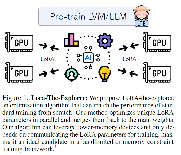
3. Method

• standard training performance can be recovered using LoRA

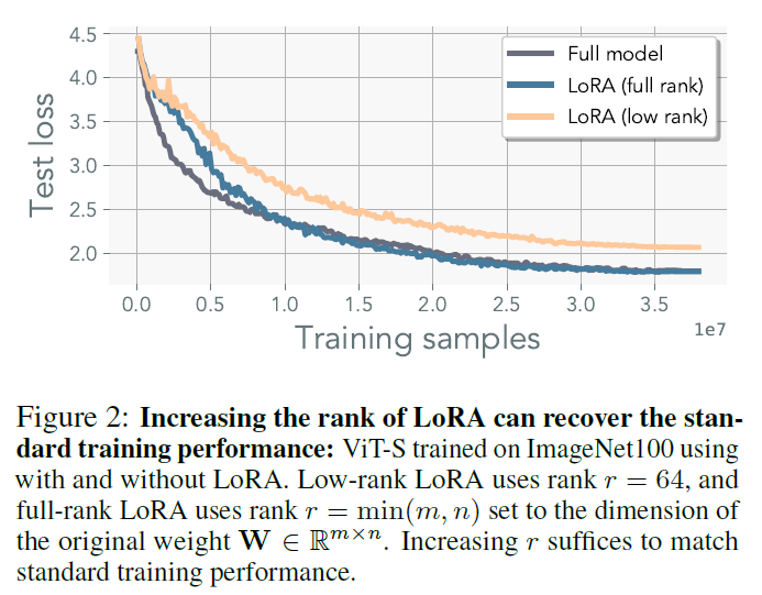
• Low-Rank LoRA shows inferior performance to the models using standard optimization

• LoRA is incapable of recovering weights that exceed the rank $r$

• Although there is a solution within a low-ranmk proximity of the initialization, it still needs the high-rank updates

3.1 Motivation : Multi-head merging perspective

• this will show why LoRA heads in parallel can achieve the performance of standard pre-training

• elevating the rank $r$ to the $\min(m, n)$ is sufficient to replicate standard pre-training performance

  • it compromises the memory efficienty of low-rank adapters

• leveraging multiple low-rank adapters in parallel

  • given a matrix of the form $\mathbf{BA} \in \reals^{d_1 \times d_2}$ and $\mathbf{B} \in \reals^{d_1 \times d}$, $\mathbf{A} \in \reals^{d \times d_2}$

  • then it is possible to represent the product as two lower-rank matrices $\mathbf{B_1A_1} + \mathbf{B_2A_2}$

    • let $\mathbf{b}_i$ and $\mathbf{a}_i$ be the column vectors
    • then we can construct $\mathbf{B_1} = [\mathbf{b}_1, ..., \mathbf{b}_{[d/2]}]$, $\mathbf{B_2} = [\mathbf{b}_{[d/2]}, ..., \mathbf{b}_{d}]$ and $\mathbf{A_1} = [\mathbf{a}_1^{\top}, ..., \mathbf{a}_{[d/2]}^{\top}]$, $\mathbf{A_2} = [\mathbf{a}_{[d/2]}^{\top}, ..., \mathbf{a}_{d}^{\top}]$
    • then this approximates the high-rank matrix into a linear combination of low-rank matrices
    • the same comclusion can be reached by beginning with a linear combination of rank-1 matrices
    • This forms the basis for a novel multi-head LoRA

Multi-head LoRA (MHLoRA)

• given a matrix $\mathbf{W} \in \reals^{m \times n}$ and constant $N$

• $f_{\text{mhlora}}(\mathbf{x}) = \mathbf{Wx} + {s \over N} \displaystyle\sum^N_{n=1} \mathbf{B}_n \mathbf{A}_n \mathbf{x}$

• reparameterizes full rank weights into a linear combination fo low-rank weights

• single parallel LoRA head can approximate the trajectory of a single step of the multi-head LoRA given that the parallel LoRA heads are periodically merged into the full weights

  • using the same rank $r$ for all the LoRA parameters
  • $\argmin_{\mathbf{B}_n \mathbf{A}_n} \mathcal{L} \left( \mathbf{W} + {s \over N} \displaystyle\sum ^N _{n=1} \mathbf{B}_n \mathbf{A}_n\right) = \argmin_{\hat{\mathbf{B}}_n \hat{\mathbf{A}}_n} \mathcal{L} \left( \hat{\mathbf{W}} + {s \over N} \hat{\mathbf{B}}_n \hat{\mathbf{A}}_n\right)$
  • used hat for the single parallel LoRA head
  • when either $\sum_{n=1}^N = \mathbf{B}_n \mathbf{A}_n = \hat{\mathbf{B}}_n \hat{\mathbf{A}}_n$ or $\hat{\mathbf{W}} = \mathbf{W} + {s \over N} \sum _{j \not = n}^N \mathbf{B}_j \mathbf{A}_j$

• The first scenario is rank deficient $\rightarrow$ unable to recover the original model performance

• The latter case necessitates that $\hat{\mathbf{W}}$ accumulates all the information of the LoRA parameters at every iteration $\rightarrow$ if we use a merge operator at every iteration, recovering the exact update is possible

• one can recover the exact gradient updates of the MHLoRA

• in distributed setting, only the LoRA params/gradients have to be communicated across devices $\rightarrow$ good when the interconnect speed is limited

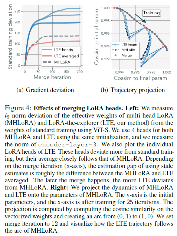
3.2 LoRA soup: delayed LoRA merging

• To reduce the communication cost of LTE

  • local updates
  • model-averaging

• allow LoRA parameters to train independently for longer period befor e merge operator

  • $\hat{\mathbf{W}} = \mathbf{W} + {s \over N} \sum _{j \not = n}^N \mathbf{B}'_j \mathbf{A}'_j$
  • $'$ for stale estimate the parameters

• Merging every iteration $\rightarrow$ ensures the representation will not diverge

• using stale estimetes relaxes this equivalence $\rightarrow$ it can still match the standard training performance

  • As its estimate is inaccurate, the optimization trajectory diverge from the optimization path of MHLoRA

  • it doesn't imply that the model won't optimize

  • just different path from MHLoRA

  • used simple averaging (left more sophisticated merging as future work)

    

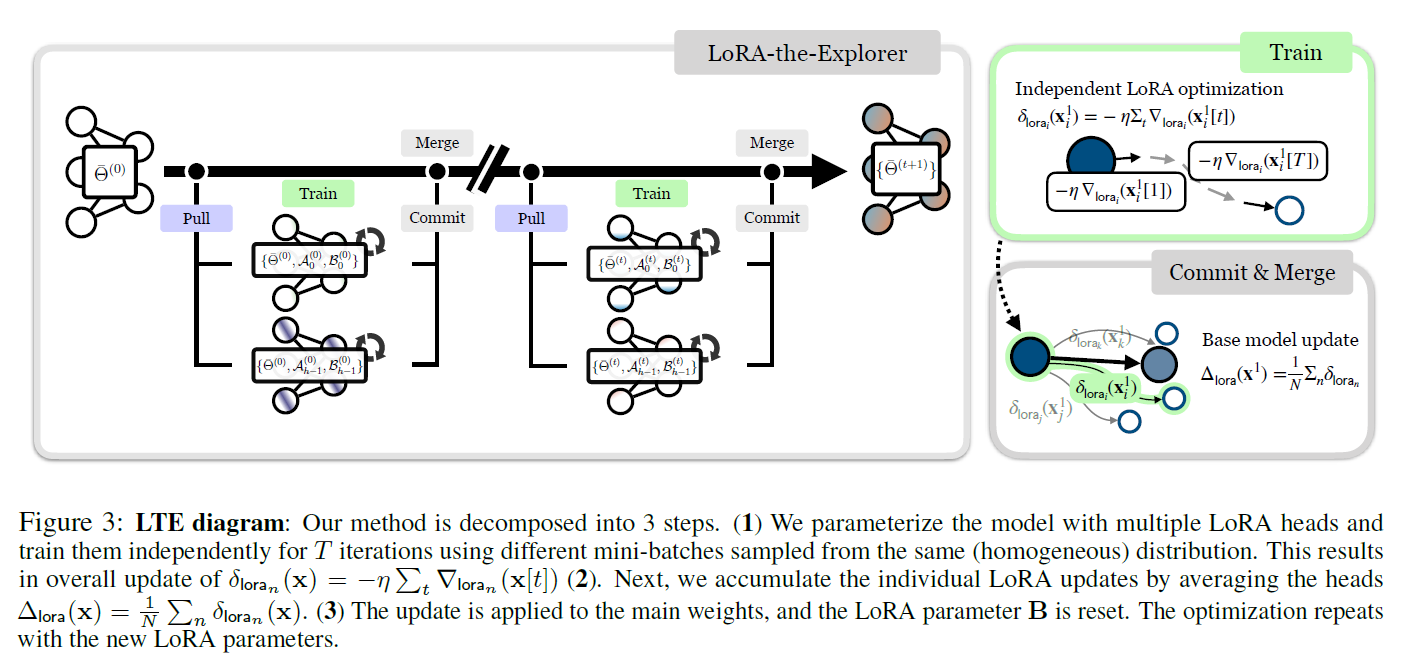
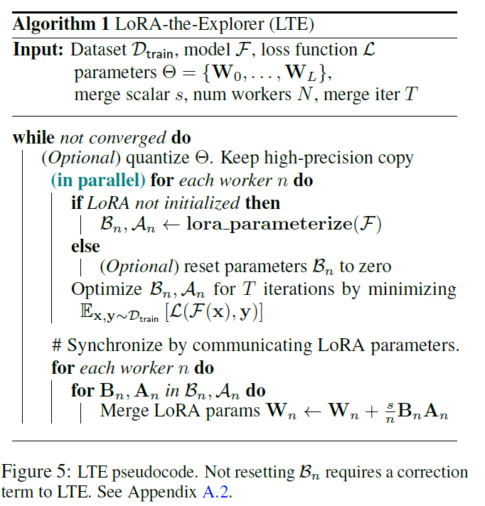
3.3 LoRA-the-Explorer: parallel low-rank updates

• achieving an informative update $\Delta \mathbf{W}$ that does not require materialization of the full parameter size during training

• parameterizing $\mathbf{W}$ such that it can be stored in low-precision and communicated efficiently (using quantized weights and keeping a high-precision copy)

• LoRA-the-Explorer (LTE) : optimization algorithm that approximates full-rank updates with parallel low-rank updates

  • creates $N$-different LoRA for each linear layer at initialization

  • each worker is assigned the LoRA parameter and creates a local optimizer

  • independently sample data from the same distribution $\mathbf{x} = \{ \mathbf{x}_1, ..., \mathbf{x}_N\}$

  • for each LoRA head $n$, optimize the parameters with own partition for $T$ iterations to get $\delta_{\text{lora}_n} = -\eta \sum_{t=1} ^T \nabla_{\text{lora}_n} \mathbf{x}_i[t]$

  • don't synchronize the optimizer state across workers

  • After the optimization, synchronize the LoRA parameters to compute the final update for the main weight $\Delta_{\text{lora}}(\mathbf{x}) = {1 \over N} \sum_{n=1}^N \delta_N$

  • then update the LoRA parameters with the updated weights $\mathbf{W}$

    • re-initialize the LoRA parameter or use the same value with correction term

  • since it doesn't train directly on the main parameter $\mathbf{W}$, using quantized parameter $q(\mathbf{W})$ is possible

    • keep the high-precision weight only in the master node or offload it from device during training

3.4 Implementation details

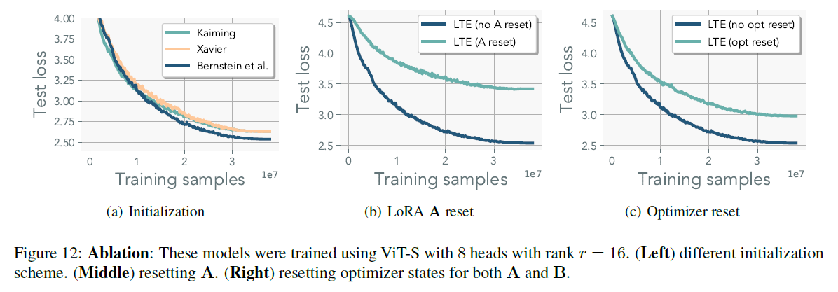
Not resetting matrix A and optimizer states

• investigated whether the matrices $\mathbf{A}_n$ would converge to the same sub-space during training
  • If so, resetting $\mathbf{A}_n$ or using regularizer are needed
  • $\mathbf{A}$ is orthogonal to remain consistent throughout training
  • without reset, it performed better (re-learning $\mathbf{A}$ and re-accumulating the optimizer are wasting optimization steps)
    

scaling up $s$ and lowering learning rate $\eta$

• scaling $s$ has the same effect as tuning the lr $\eta$ $\rightarrow$ common misconception

• during experiment, there is no comparable performance when using $s$ to be 1~4

  • using large $s$ and slightly lowering $\eta$ worked best

  • standard practice : set $s$ proportional to the rank $r$, i.e. $s = {\alpha \over r}$

  • used $\alpha = 4096, s = 64$ and $\eta = 2 \cdot 10^{-4}$

  • lr doesn't scale linearly with $s$

  • $s$ only affects the forward computation

    • it modifies the contribution of the LoRA parameters in the forward pass $\rightarrow$ implacation on the effective gradient

  • $s$ scales quadratically with the alignment of $\bold{B}$ and $\bold{A}$

Significance of Initialization Strategies

• used the initialization scheme that utilizes a semi-orthogonal matrix scaled by $\sqrt{d_{out}/d_{in}}$
  • originally designed for standard feed-forward models
  • whereas LoRA operates under the assumption that $\bold{B}$ is zero-initialized with a residual connection
  • in Ablation study, Kaiming initialization and Xavier initialization performing similar

4. Experiments

• in transformer experiment, they misused the scaling factor $1/\sqrt{d_{out}}$ instead of the standard scaling $1/\sqrt{d_{out}/n_{attn}}$ (they will revise the hyper-parameter)

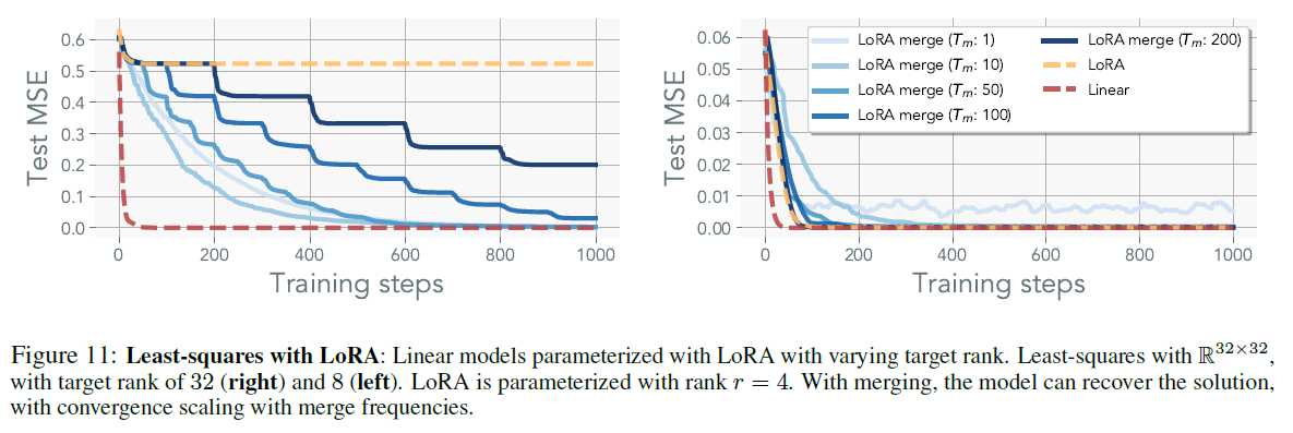
4.1 Iterative LoRA Merging

• iteratively merging LoRA is a key component in recovering the full-rank representation

• they assess the effectiveness of merging a single LoRA head in context of linera networks trained on synthetic LS regression datasets
  

• without merging, the model performance is not changing

• iterative merging recovers the GT solution with the rate increasing with higher merge frequency

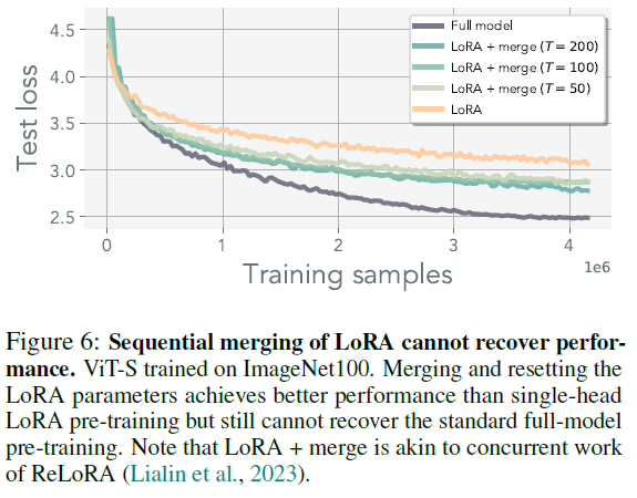
• in Vit-S with patch size 32 on ImageNet100
  • merging of a single LoRA head outperforms standalone LoRA
  • frequent merging delays convergence (LoRA parameter re-initialization and momentum state inconsistencies)
  • performance doesn't match $\rightarrow$ potential local minima when training with rank-deficient representation
• they found the merge iteration of $T = 10$ is still stable when using batch size of 4096
  • with higher $T$, additional training may be required
• with increased merge iteration, smarter merging techniques may be necessary

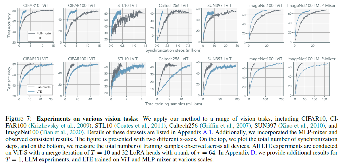
• to further test the generalizability, they conducted various vision tasks on MLP-Mixer

4.2 LoRA parameter alignment

• the efficacy of their optimization algorithm
  • individual heads to explore distince subspaces within the parameter space
    
  • average cosine similarity and Grassman distance between the heads $\bold{B}_n \bold{A}_n$
  • conducted with data samples drawn from same distribution
  • each set of LoRA parameters was exposed to a different set of samples
  • LoRA heads do not converge to the same representation
  • this orthogonality is maximized when using different parameters and different data (mini-batches)

4.3 Ablation study: the effect of LoRA heads, rank, and merge iteration

• monotonic improvement in performance with an increased number of heads and ranks

• extending the merge iteration negatively impacts performance

• in LS regression, excessive merging hurts model accuracy

• with large enough rank and head, the model converges to better accuracy even if the test loss was similar

• averaging of the LoRA heads has a regularization effect similar to model ensembling

• ViT-S as the primary architecture

  • hidden size = 384
  • MLP dimension = 1536
  • number of heads * rank of the LoRA > the largest dimension of the model $\rightarrow$ worked well
  • number of heads > rank $\rightarrow$ longer iterations were required

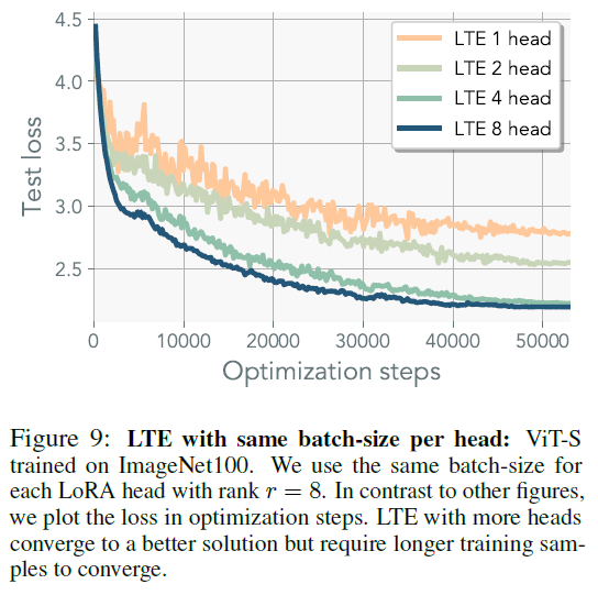
4.4 Gradient noise with parallel updates

• in ablation, they fixed cumulative batch size of 4096 and epoch of 1200

• each LoRA head received a reduced batch size of 4096/heads

• scaling the rank exerts a greater impact than increasing the number of heads

  • proportional scaling of gradient noise with smaller mini-batches

  • gradient noise contribute to slower convergence in addition to the use of stale parameter estimates

    

  • increasing the number of heads necessitates more sequential FLOPs but it offers efficient parallelization

• using a larger batch size for gradient estimation may prove beneficial in distributed training

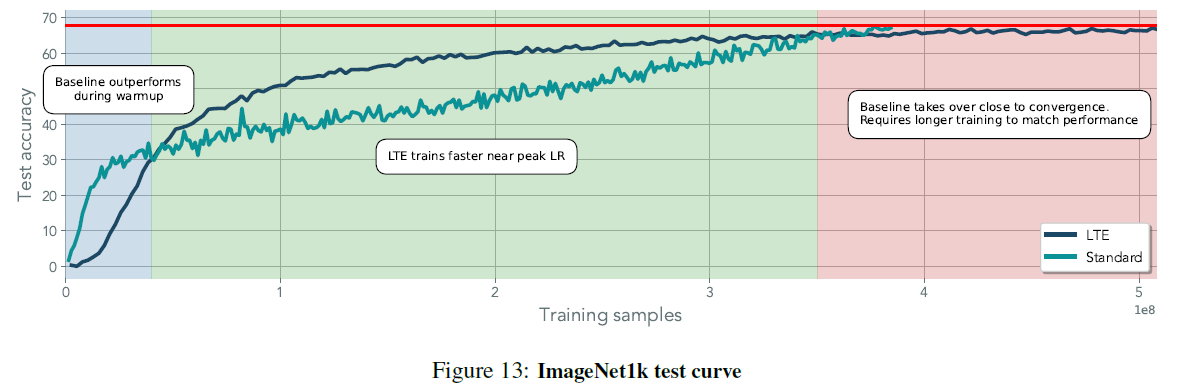
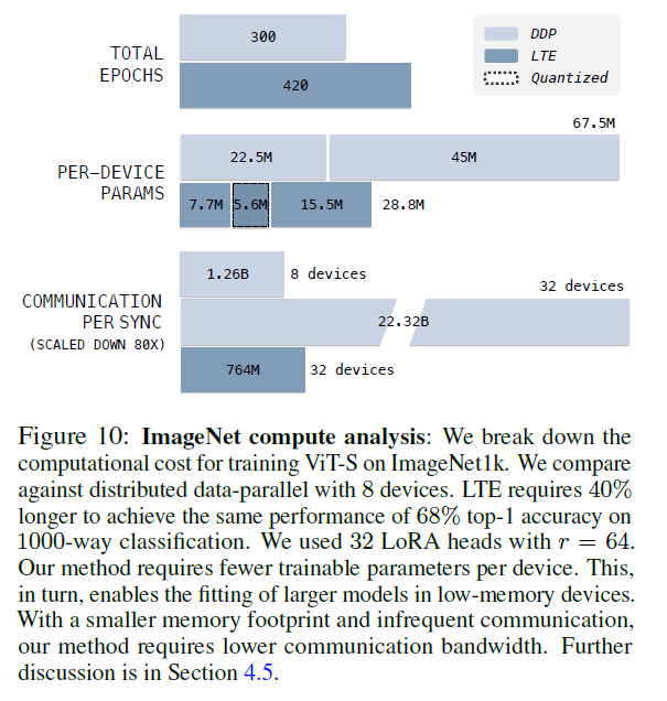
4.5 Performance Scaling on ImageNet-1K

• scaled up to ImageNet 1K
  • doubled batch size to 8192
  • didn't changed the way mini-batches were sampled
  • scheduling the randomness for the mini-batches is not explored
• in Initial training, LTE outperformed standard training
  • as training completed, standard training overtook LTE
  • LTE needs additional iterations to achieve comparable performance
• standard training appeared to benefit more from a lower lr compared to LTE

• this study is focused on training deep networks with parallel low-rank adapters (not efficiency!)

• hypothetical computation analysis for future scaling efforts

  • model size $M_{\text{ddp}} = M$ and $M_{\text{lte}}$ for LTE

  • the number of devices for each method $N_{\text{ddp}}$ and $N_{\text{lte}}$

  • with quantization, each LTE device require a memory footprint of $qM + M_{\text{lte}}$

  • as base model is 16-bit and if we use 4-bit quantizing, $q = 0.25$

  • with AdamW, DDP necessitates an additional $2M$ parameters (total $3M$)

  • for LTE, $qM + 3M_{\text{lte}}$ is needed

  • Assuming the training is parameter bound by the main weights $r << \min(m, n)$, LTE can leverage GPUs roughly 1/3 size of DDP

  • LTE requires 40% more data and 20% slowdown per iteration with quantization (QLoRA)

  • on average, each LTE device observes 1/3 less data than a device in DDP

    

  • Communication bottleneck

    • In multi-node systems, the communication scales with the size of the model and is bottlenecked at interconnect speed
    • using standard all-reduce, the gradient shared between each device for a total communication of $N_{\text{ddp}}(N_{\text{ddp}} - 1)M$
    • for LTE, as it communicate every $T$ iteration so ${1 \over T}N_{\text{lte}}(N_{\text{lte}} - 1)M$
    • using parameter server method (1 and broadcast), gradients are sent to the main parameter server and averaged
    • DDP with a parameter server would use $2(N_{\text{ddp}}-1)M$
    • LTE with parameter server would use ${1 \over T}(N_{\text{lte}} - 1)(qM + M_{\text{lte}})$
    • LTE can leverage lower-bandwidth communication as the parameters shared between devices are strictly smaller by a factor of $M_{\text{ddp}}/M_{\text{lte}}$

5. Related works

• Training with adapters

  • LoRA
  • MoE PEFT and averaging
  • Additive adapters
  • Adapters for NLP, vision, video, incremental learning, domain adaptation, vision-language, text-to-vision, perceptual learning

• Distributed Training and Federated Learning

  • Federated Learning in low-compute devices, high-latency training, privacym, cross and in-silo learning
  • communication efficiency
    • local steps
    • decentralized training
    • gradient checkpointing
    • reversible gradient computation
    • gradient or weight compression
  • Combining models in federated learning
    • FedAvg
    • weight averaging
    • probabilistic frameworks for merging
    • updating with stale parameters
  • Server momentum and adaptive methods
  • bi-level optimization schemes

• Linear mode connectivity and model averaging

  • deep models can be connected through nonlinear means
  • linear paths with constant energy exist in trained models
  • for models with different initialization, parameter permutations can be solved to align them linearly
  • model averaging
  • model stitching
  • Anna Karenina principle
  • model averaging within ensembles
  • utilizing an average model as a target

6. Conclusion

• Low-rank adapters for model pre-training

• LTE : bi-level optimization method that capicalizes on the memory-efficient properties of LoRA

• how to accelerate convergence during the final 10% of the training?

• how to dynamically determine the nuimber of ranks or heads?

• is heterogeneous parameterization of LoRA feasible where each LoRA has a different rank?

• what strategies for merging can achieve higher performance?

• This study is showing viability

• tests on larger models are needed

• this will pave the way for pre-training models in computationally constrained or low-bandwidth environments

  • less capable and low-memory devices can train a large model
  • wisdom of the crowd

7. Comment

메인 파라미터들을 건드리지 않고 어댑터를 이용해 전체 모델을 근사하여 복원한다는 아이디어. rank r의 LoRA를 다시 rank 1로 decompose하여 바로 합치는 것이 아니라 주기적으로 병합해주는 것. 왜 lora를 다시 분해한다는 생각은 안해봤을까.