[CV] 9. Image Segmentation

Week 9-2. Image Segmentation

1. Segmentation by Humans

2. K-Means Segmentation

• Pixels in Euclidean Space: Pixels as feature vectors: [R, G, B, x, y, ...]
  고차원 상에서 픽셀 위치 있음, 유사도 측정해서 cluster

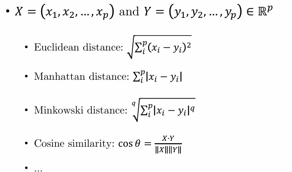
• Similarity Measure
  문제의 특징에 따라 골라야 함, 결과 많이 달라짐

K-Means Clustering
1. Choose the number of clusters k
2. Initialize cluster centers (centroids) $\mu_1, \mu_2,...,\mu_k$
• e.g., Could pick k feature points and set cluster centers to these points
3. For each feature point, compute the cluster center it is closest to
(using some distance measure) and assign the feature point to this cluster
4. Re-compute cluster centers (mean of data points in the cluster)
5. Repeat 3 and 4 until meet the stop condition

3. Mean Shift Segmentation

4. Graph Cut Segmentation

Images as Graphs
node- pixel
edge (p,q)
Graph notation: G = (V,E)
Affinity weight $w_{pq}$ for each edge

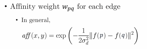
시그마: 하이퍼 파라미터- 높아질수록 0에 천천히 가까워짐, 멀리 있어도 어느정도 높게 나옴

• edges

  • Fully connected:
  Captures all pairwise similarities
  Infeasible for most images
  • Neighboring pixels:
  Very fast to compute
  Only captures very local interactions
  • Local neighborhood: 얼마나 떨어진 애들까지 연결할지(절충안)
  Reasonably fast, graph still very sparse
  Good tradeoff
  연결 안하면 affinity weight = 0

Segmentation by Graph Cuts
Break Graph into Segments

Minimum Cut

Cut C = (A,B)는 그래프의 vertices(nodes)를 subsets A, B로 나누는 것
Cut-Set: 다른 subset에 있음
Cost of Cut: Sum of weigths of cut set edges

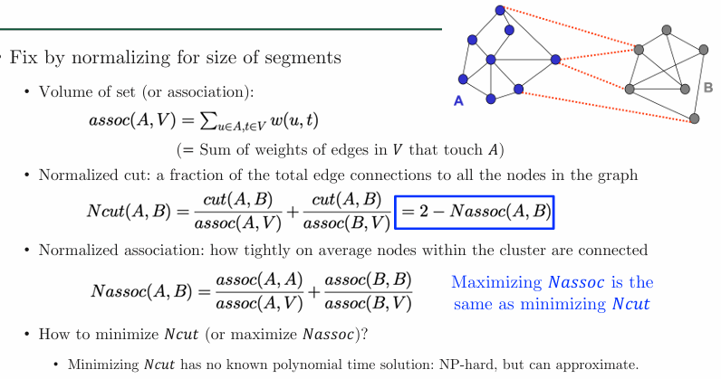
Normalized Cut

• Fix by normalizing for size of segments
  cut/A + cut/B = 2-(A/A + A/B)
  minimize Ncut = maximize Nassoc

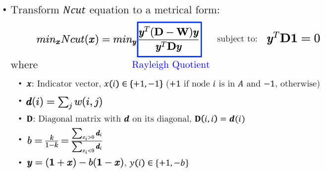
• Transform Ncut equation to a metrical form
  x \in {+1, -1}
  y \in {+1, -b}
  엄밀히 말하면 y = /2
  matrix w: diagonal 0
  minimize하는 y 찾기
  편하게는 $x^T(-w)x$
  1xN(NxNNx1) = 1xNNx1 = 1
• 6 4 -> 6 4
  6 + cut +1 +1 -1 6+
  4 cut - -1 4-
  cut 낮을수록 좋음

• solution is given by the generalized eigenvalue problem
  $Ax = \lamda x$
  $A\lamda = \lamda Bx$
  $(D - W)y = \lamda Dy$
  Optimal solution: second smallest eigenvector

Recursive Normalized Cut
weighted graph: G = (V,E)
Solve the eigenvalue problem: $(D - W)y = \lamda Dy$
Use the eigenvector with the second smallest eigenvalue to bipartition the graph
Note: this is an approximation
Recursively repartition the segmented parts if necessary
affinity: 친화성,인척 관계

Normalized Cut: Comments
Pros
• Generic framework can be used with many different features and affinity formulations
• Generally works better than other methods we have seen so far
Cons
• Need to choose a number of segments
• High storage requirement and time complexity
• Bias towards partitioning into equal segments