[ML] 7. Principal Component Analysis (PCA)

Week11. Unsupervised Learning: Principal Component Analysis (PCA)

dimension reduction
to understand key features, the most variance in data set (high variance high importance)
visualization, data analysis
create new dimensional components that are combinations of proportions of the existing featrues; transformation

Theory and Intuition

• Dimension Reduction
  help visualize and understand complex data sets
  act as a simpler data set for training data
  reduce N features to a desired smaller set of components through a transformation, not simply select a subset of features

• Variance explained
  Certain features are more important than other features
  unlabeled data, determine feature importance?

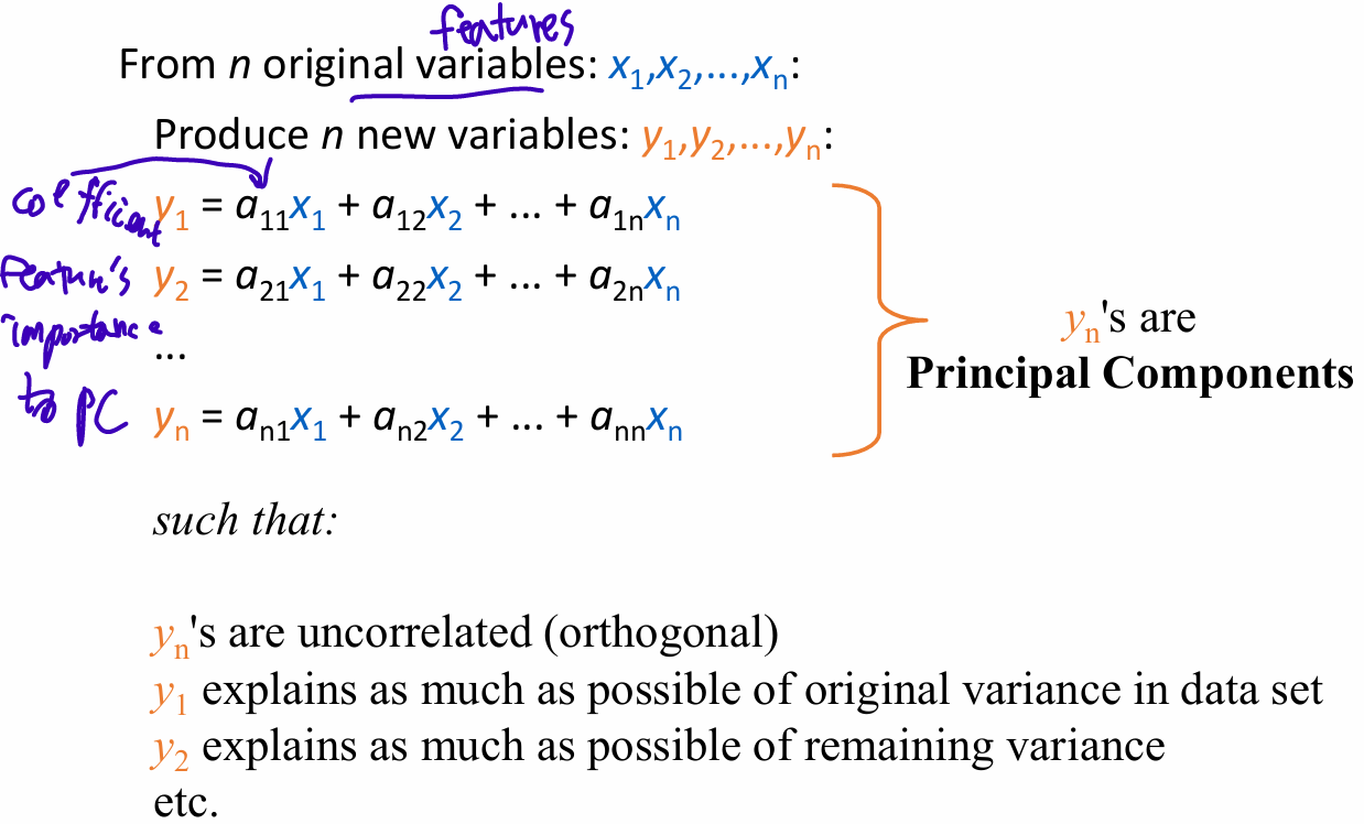
• Principal Component: a linear combination of original features

The more variance the original features accounts for, the more influence it has over the principal components
This single principal component can explain some percentage of the original data like 90%.
trade off some of the explained variance for less dimensions (low explained variance, low dimenstion)

Math

creating a new set of dimensions (the principal components) that are normalized linear combinations of the original features
$Z_1 = \phi_{11}X_1 + \phi_{21} X_2 + ... + \phi_{p1} X_p$

• standardize the data

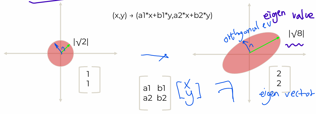
• Linear transformation of data
• EigenVector: Directional information
• EigenValue: Magnitude information
• Orthogonal Eigenvector

• Apply Linear Transformation
• EigenValue measures variance explained

PCA STEPS
○ Get original data
○ Calculate Covariance Matrix
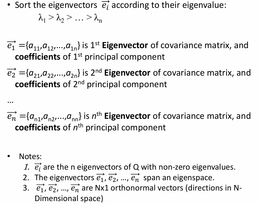
○ Calculate EigenVectors
○ Sort EigenVectors by EigenValues
○ Choose N largest EigenValues
○ Project original data onto EigenVectors

Recap: PCA Steps

• Data preprcessing
  $\displaystyle \mu_j = \frac{1}{m}\sum^m_{i=1} x_j^{(i)}\\ x_j^{(i)} = x_j - \mu_j$ replace
• Ader normalization and optionally feature scaling,
• Compute "covariance matrix":
  Sigma = $\displaystyle \frac{1}{m}\sum^n_{i=1}(x^{(i)})(x^{(i)})^T$
• Compute "eignevectors" of matrix Sigma:

[U,S,V] = svd(Sigma);
Ureduce = (:, 1:k);
z = Ureduce'*x;

$z = U^T_{reduce}x$

Background: Covariance
Measure of the “spread” of a set of points around their center of mass(mean)

• Variance: Measure of the deviation from the mean for points in one dimension
• Covariance: Measure of how much each of the dimensions vary from the mean with respect to each other
  measured, relation between two dimensions
  covariance between one dimension is the variance
  $\displaystyle var(X) = \frac{\sum^n_{i=1}(X_i - \bar{X})(X_i - \bar{X})}{(n-1)}, \;cov(X,Y) = \frac{\sum^n_{i=1}(X_i - \bar{X})(Y_i - \bar{Y})}{n-1}$

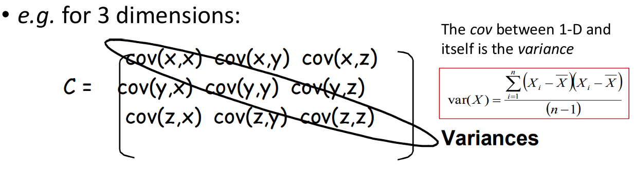
cov(x,y) = cov(y,x) symmetrical about the diagonal
N-dimensional data; NxN covariance matrix

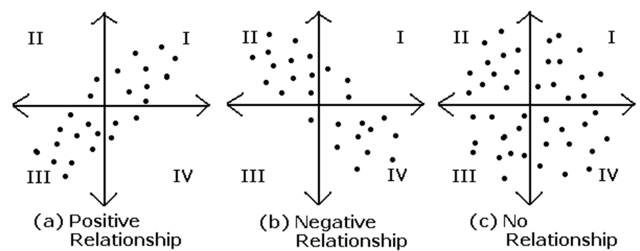
• value
  positive value; both dimensions increase or decrease together
  negative value; while one increases the other decreases
  zero; two dimensions are independent of each other

PCA
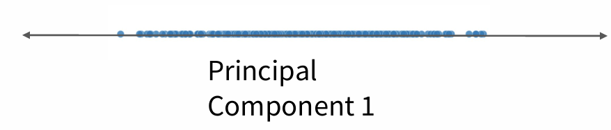
PCA is used to simplify a dataset, reduce dimensionality by eliminating the later principal components.
It is a linear transformation that greatest variance comes to the first axis, the first principal component, the scond greatest variance on the second axis, and so on.

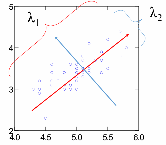
• Principal components
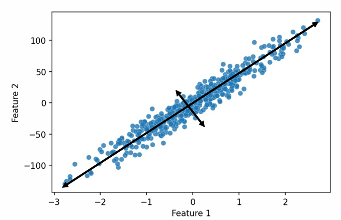
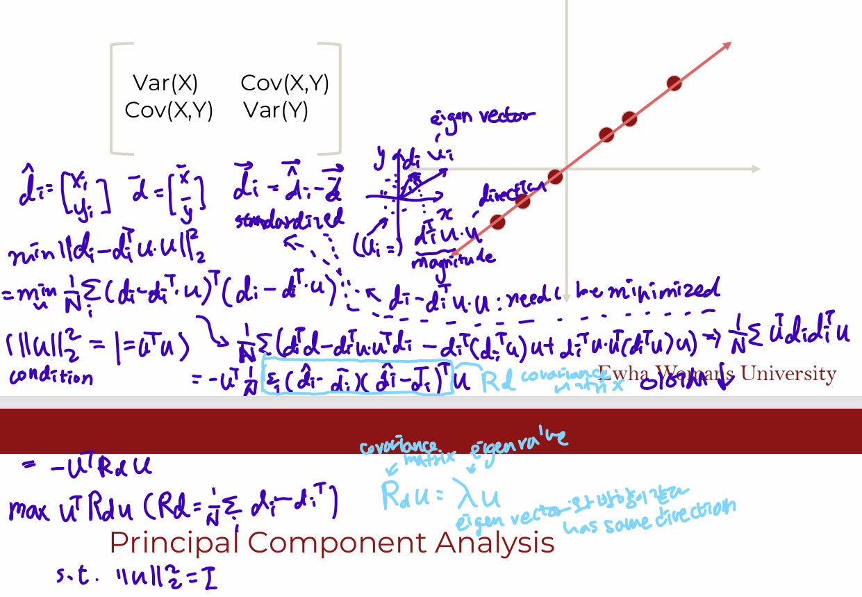
  First PC is direction of maximum variance from origin
  Subsequent PCs are orthogonal to first PC and describe maximum residual variance

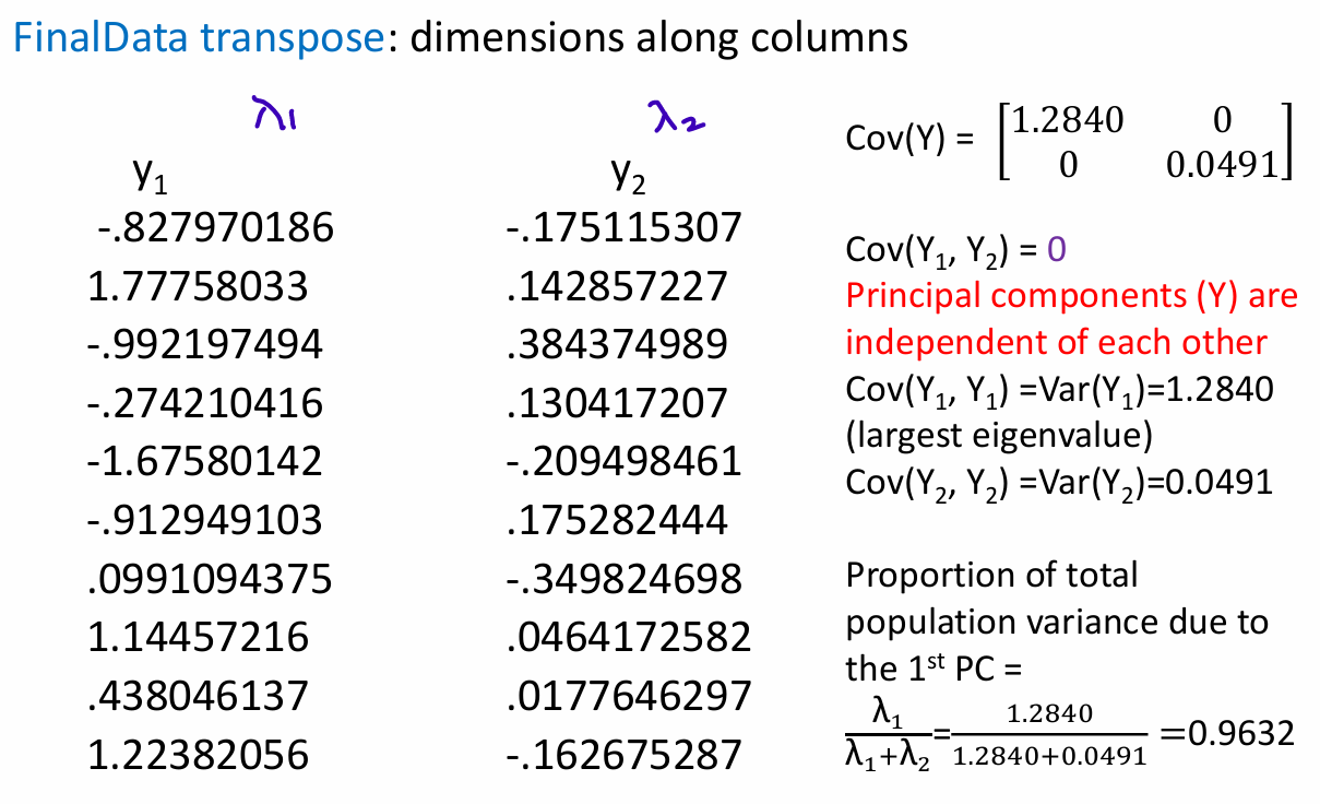
• Eigenvalues of the covariance matrix = Variances of each principal component
  find largest eigenvalues
  

• Application: face recognition and image compression, finding patterns in data of high dimension

PCA Theorem

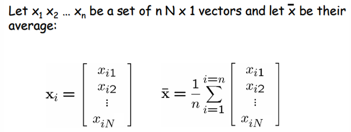
• Let X be the N x n matrix with columns:
  $X = [x_1 - \bar{x}\; x_2 - \bar{x}\; ...\; x_n - \bar{x}]$

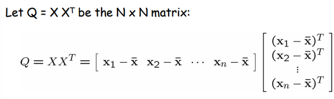
Q is square, symmetric, the covariance matrix(scatter matrix), can be very large

• Expressing x in terms of e1...en has not changed the size of data
  However, if the points are highly correlated, x will be close to zero; they lie in a lower-dimensional linear subspace

PCA Example

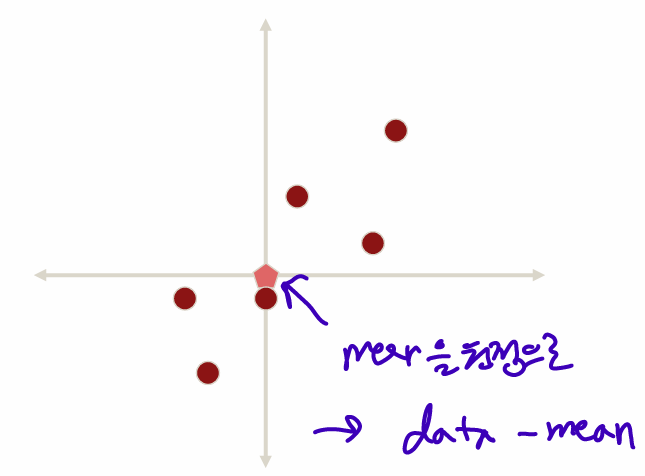
1. Substract the mean
   $x_i = x_i - \bar{x}$, mean으로 원점이동

2. Calculate the covariance matrix
   cov = $\begin{pmatrix} .6165\; .6154\\ .6154\; .7165\end{pmatrix}$
   Non-diagonal elements are positive; $x_1, x_2$ variable increases together

3. Calculate the eigenvectors and eigenvalues of the covariance matrix
   eigenvalues = $\begin{pmatrix} .0490; 1.2840\end{pmatrix}$
   eigenvectors = $\begin{pmatrix} -.7351\; -.6778\\ .6778\; -.7351\end{pmatrix}$

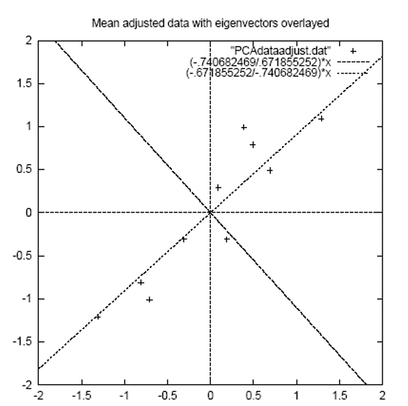
perpendicular to each other, first line is of best fit

4. Reduce dimensionality and form feature vector

The eigenvector with the highest eigenvalue is the principal component of the data set.
Order eigenvectors by eigen value, highest to lowest, in order of significance.
Ignore the components of lesser significance, lose some information
choose only the first p eigenvectors; final data set has only p dimension

• Feature Vector = (eig1 eig2 eig3 ... eign)
  leave out less significant component and only have a single column
  $\begin{pmatrix} -.7351\; -.6778\\ .6778\; -.7351\end{pmatrix}$ to $\begin{pmatrix} -.6778\\ -.7351\end{pmatrix}$

5. Deriving the new data

FinalData = RowFeatureVector x RowZeroMeanData
RowZeroMeanData = RowFeatureVector$^{-1}$ x Final Data
RowOriginalData = (RowFeatureVector$^{-1}$ x FinalData) + Original mean

RowFeatrueVector: eigen vectors in the columns transposed, eigenvecors in rows with the most significant eigenvector at the top
RowZeroMeanData: the mean-adjusted data transposed, data items in column, each row holding a seperate dimension

• FinalData transpose