[ML] 8. Naive Bayes (NB)

Week 12. Naive Bayes

Supervised Learning text tasks, classification
Naive Bayes and NLP (use raw string text)

1. Bayes' Theorem

$\displaystyle P(A|B) = \frac{P(B|A)\cdot P(A)}{P(B)}$
P(A|B) is probability of event A given that B is True. (B가 True일 떄 A가 True일 확률)
P(B|A) is probability of event B given that A is True. (A가 True일 떄 B가 True일 확률) Likelihood
P(A) is probability of A occurring.
P(B) is probability of B occurring.
$\displaystyle posterior = \frac{prior \times likelihood}{evidence}$

• Example: fire alarm detection system
  actual dangerous fires 1%; P(fire)
  smoke alarms 10%; P(alarm)
  actual dangerous fire, smoke alarm 95%; P(alarm|fire)
  P(fire|alarm) = 95 1 / 10 = 9.5% (P(alarm|fire)P(fire) / P(alarm))

2. Naive Bayes

Math
$\displaystyle posterior = \frac{prior \times likelihood}{evidence}$

$\displaystyle p(C_k|x) = \frac{p(C_k)p(x|C_k)}{p(x)} = \frac{p(C_k, x_1,...,x_n)}{p(x)}$
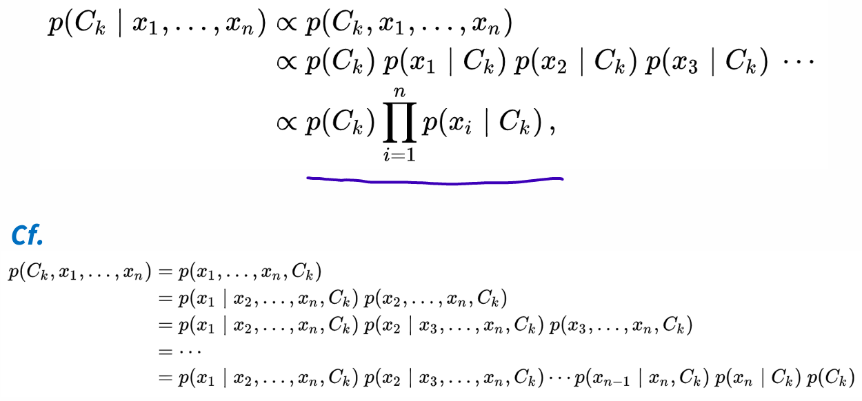
The joint probability can be decomposed into a product of conditional probabilities
Assume all X features are mutually independent of each other

Multinomial Naive Bayes
Example: classify movie reviews into positive and negative
labeled data set
simple count vectorization model (counting the frequency of each word in each document) 문서에서 단어 몇번 나왔는지 셈

• Begin by seperating out document classes:
  positive 25, negative 10
• Create "prior" probalities for each classes:
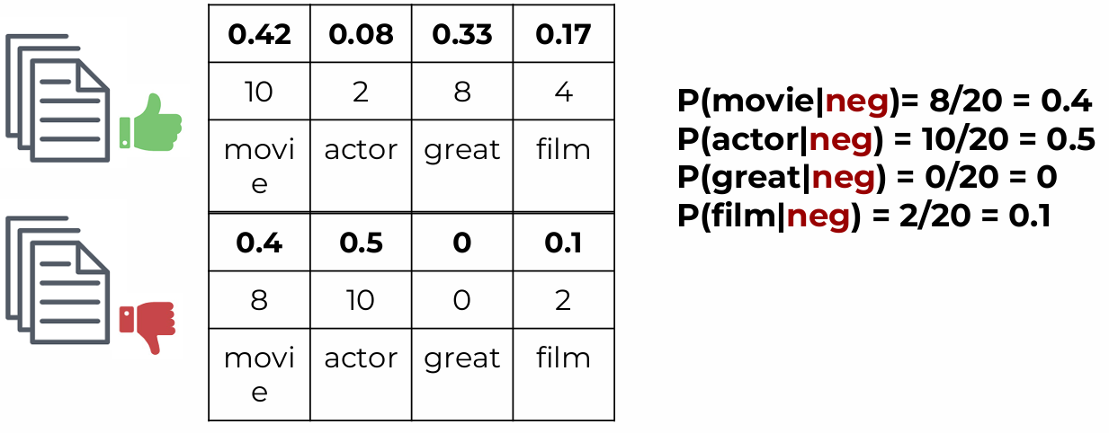
  positive 25/35, negative 10/35
• Start with count vectorization on classes:
• Calculate conditional Probabilities per class and word

• Now a new revies was created:
  "movie actor"
• Start with prior probability, continue with conditional probabilities, and calculate this score factor

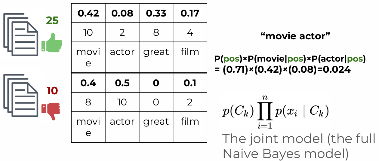
• Score is proprotional to P(pos|"movie actor")
• Repeat same process with negative class;
  score(P(neg)×P(movie|neg)×P(actor|neg))
  is proportional to P(neg|"movie actor")
• Compare both scores against each other
  0.057 $\propto$ P(neg|"movie actor")
  0.024 $\propto$ P(pos|"movie actor")
• Classify based on highest score: This is classifed as a negative review

Smoothng

• What about 0 count words: Alpha Smoothing parameter to add counts

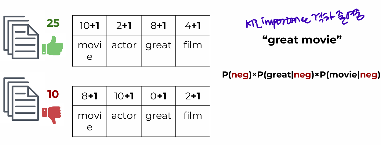
Higher alpha value will be more smoothing, giving each word less distinct importance

3. Extracting Features From Text Data

in order to pass numerical features to the machine learning algorithm

Count Vectorization

• Steps
  Create a vocabulary of all possible words
  Create a vector of frequency counts

Notice most values will be zero

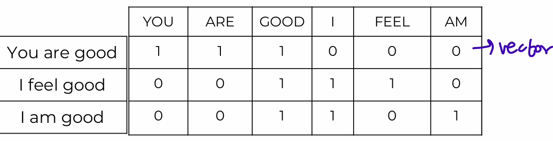
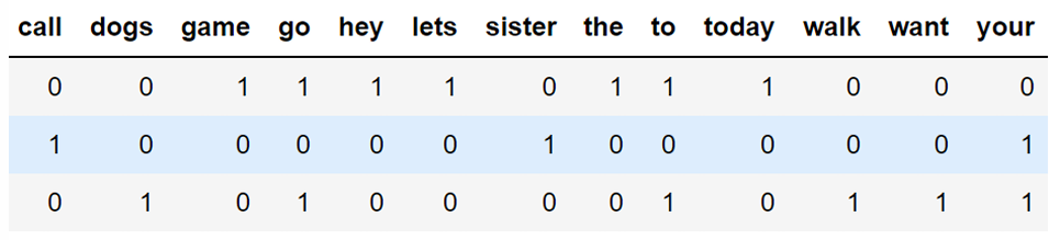
• Document Term Matrix (DTM): a mathematical matrix that shows how often terms appear in a collection of documents.

• characteristic
  treats every word as a feature, with the frequency counts acting as a strength
  sparse matrix, many zero
• Stop Words: words common enogh that safe to remove, not important, most libaraies have built-in list of them

TF-IDF Vectorization
: calculate Term Frequency-Inverse Document Frequency Value for each word
TF(T,D): term frequency, the number of times that term t occurs in document d

• Inverse document frequency factor (IDF)
  diminishes the weight of frequent termsclose to 0 and increases the weight of rare terms, How common or rare

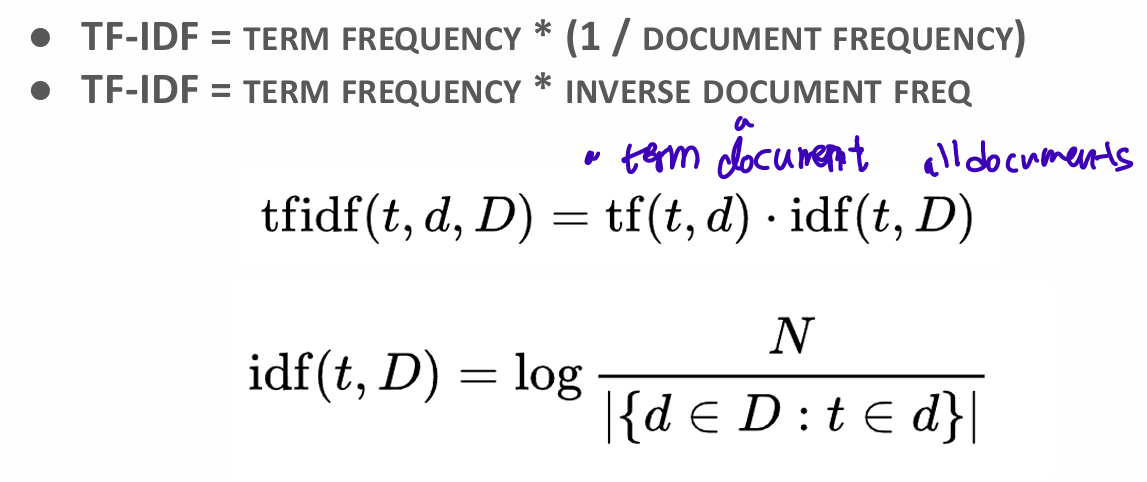
idf(t,D) = log(total number of Documents/the number of documents containing word)

• TF-IDF allows us to understand the context of words across an entire corpus of documents