선형회귀분석 실습

Data Science Python Library

• scikit-learn: Python 머신러닝 라이브러리
• numpy: Python 고성능 수치 계산을 위한 라이브러리
• pandas: 테이블 형 데이터를 다룰 수 있는 라이브러리
• matplotlib: 대표적인 시각화 라이브러리, 그래프가 단순하고 설정 작업 많음
• seaborn: matplot기반의 고급 시각화 라이브러리, 상위 수준의 인터페이스를 제공

Parameter, Attributes, Methods

• Parameter : 입력 함수 값
  ex 1) fit.intercept : bool, default = True
  ex 2) copy_X : bool, default = True
  ex 3) n_jobs : int, default = True
  ex 4) positive : bool, default = False

• Attributes : 모델이 가진 속성
  ex 1) coef : array of shape (n_features,) or (n_targets, n_features)
  ex 2) rank : int
  ex 3) singular : array of shape min(X,y),)
  ex 4) intercept : float or array of shape (n_targets,)
  ex 5) n_features_in : int
  ex 6) featurenames_in : ndarray of shape (nfeatures_in,)
  

• Methods : 지원하는 기능
  ex 1) fit(X,y[,sample_weight]) : Fit linear model. 훈련한다, 적합한다.
  ex 2) get_metadata_routing() : Get metadata routing of this object
  ex 3) get_params([deep]) : Get parameters for this estimator.
  ex 4) predict(X) : Predict using the linear model.
  ex 5) score(X,y[,sample_weight]) : Return the coefficient of determination of the prediction.
  ex 6) set_fit_request(*[, sample_weight]) : Request metadata passed to the fit method.
  ex 7) set_params(**params) : Set the parameters of this estimator.
  ex 8) set_score_request(*[, sample_weight]) : Request metadata passed to the score methods.

자주 쓰는 함수

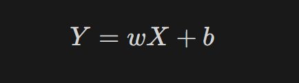
• sklearn.linear_model.LinearRegression : 선형회귀 모델 클래스
  • coef_: 회귀 계수(가중치, $w1$)
  • intercept: 편향(bias, $w0$)
  • fit: 데이터 학습(값을 넣어줘)
  • predict: 데이터 예측
  • help() : 원하는 정보를 검색
    

❗항상 fit을 먼저 사용해서 값을 넣은 뒤에 coef_, intercept등을 사용해야만 한다.

1. 키-몸무게 데이터 실습

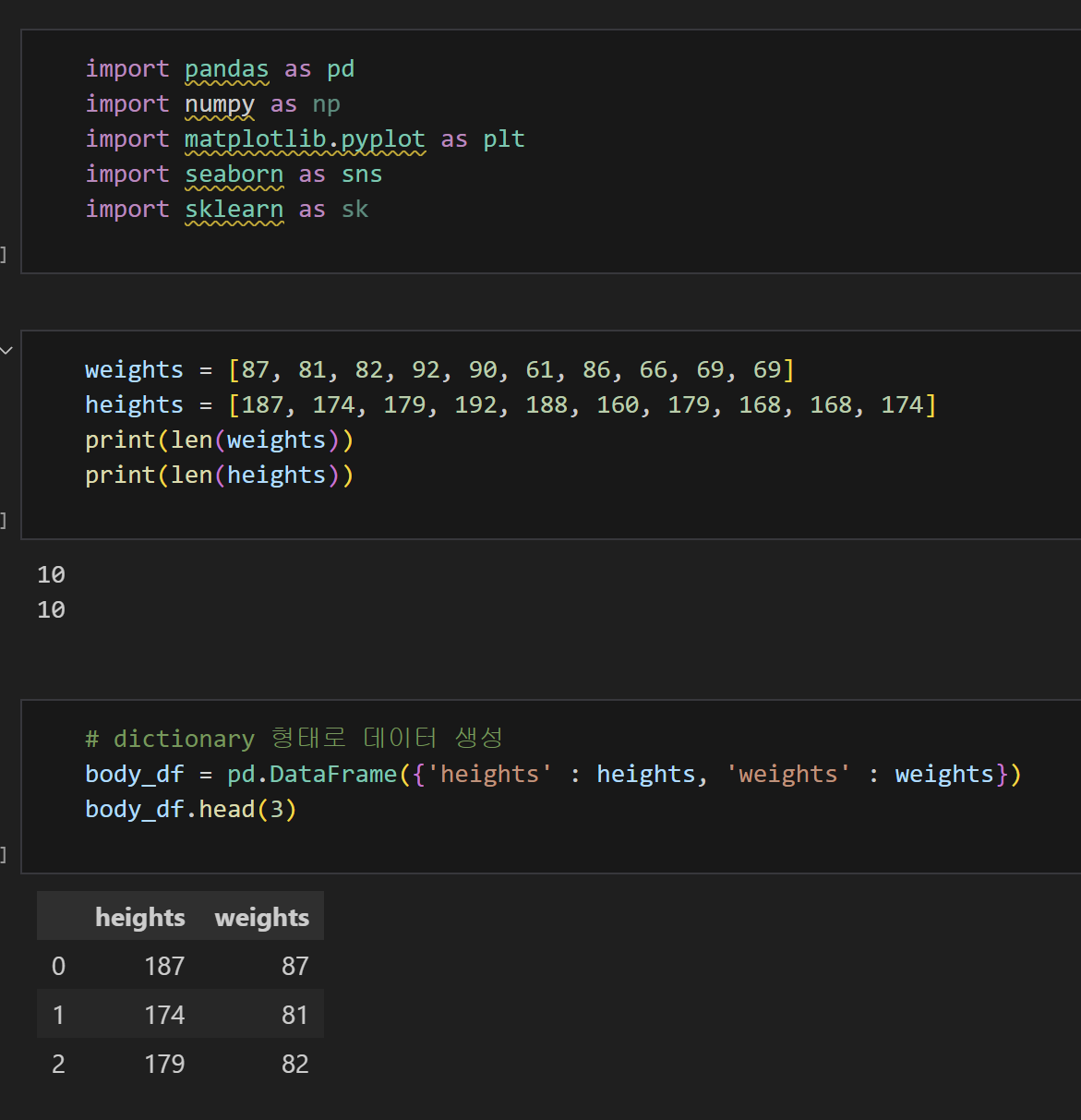
1) 데이터 생성 및 라이브러리 설치

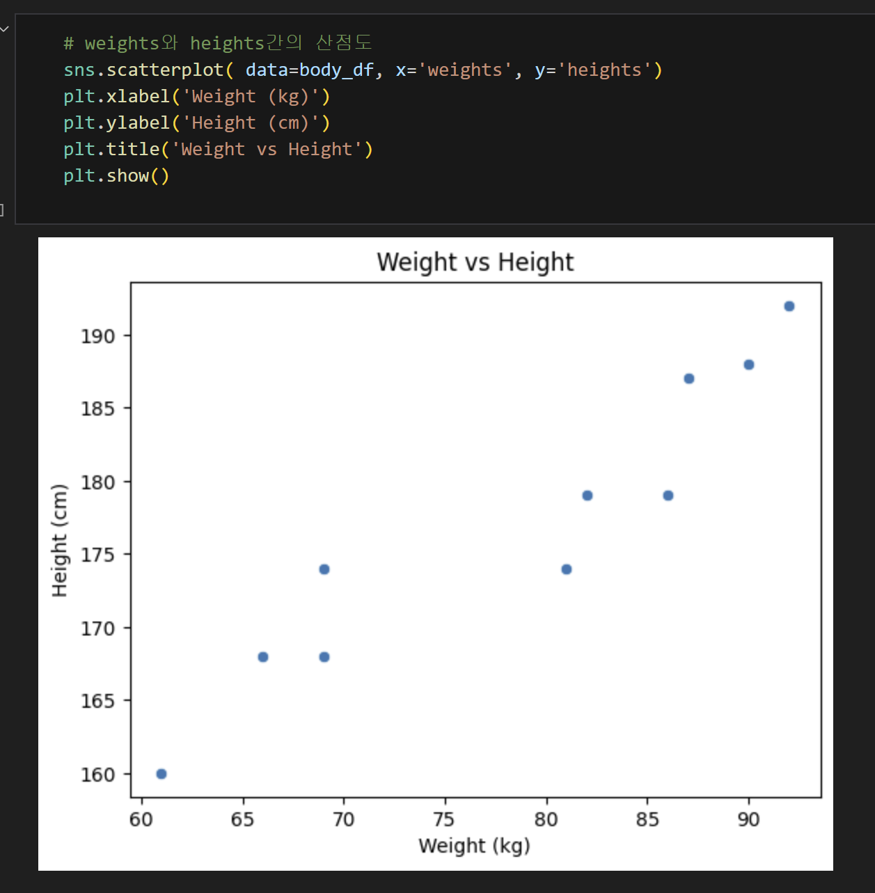
2) 산점도 확인하기

선형회귀 형태를 띄고 있다.

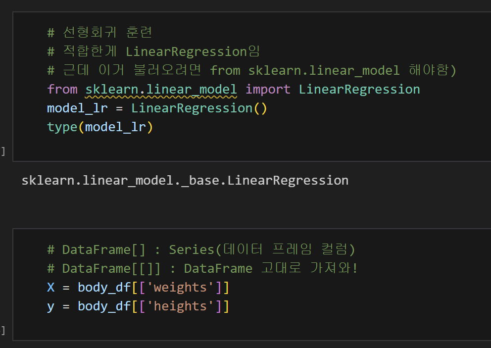
3) 선형회귀 모델 불러오고 데이터 훈련하기

from sklearn.linear_model import LinearRegression
# 선형회귀 모델 불러와줘
model_lr = LinearRegression()
# 위에 저게 너무 기니까 이렇게 줄여서 부를게
X = body_df[['weights']]
y = body_df[['heights']]
# 데이터프레임 형태 고대로 X랑 y라는 이름으로 부를게.

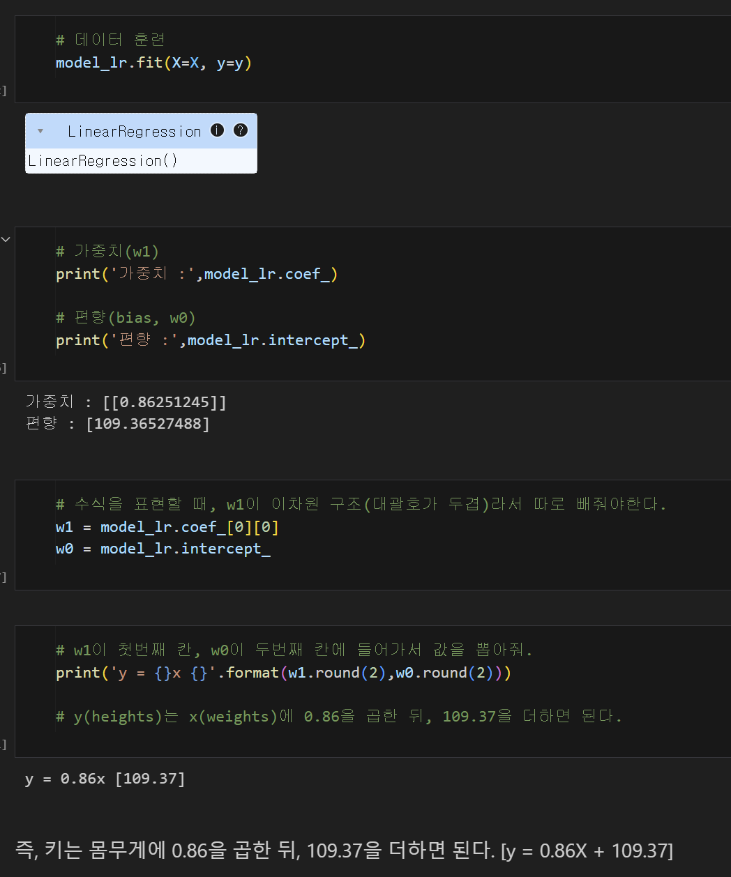
model_lr.fir(X=X, y=y)
# 선형회귀 모델을 만들건데, X값에 X라는 데이터를 넣고, y값에 y라는 데이터를 넣어.
w1 = model_lr.coef_[0][0]
# 이차원 구조니까 따로 써줄게. 근데 이거 가중치를 w1이라고 부를게.
w0 = model_lr.intercept_
# bias(편향)을 w0이라고 부를래.
print('y = {}x {}'.format(w1.round(2), w0.round(2)))
# w1을 첫번째 칸, w0을 두번째 칸에 넣어서 값을 뽑아줘.

= 즉, y(heights)는 x(weights)에 0.86을 곱한 뒤, 109.37을 더하면 된다.

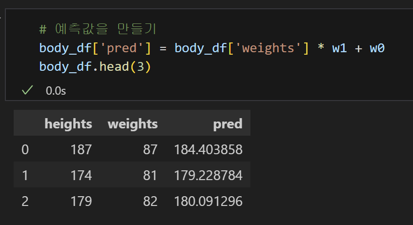
4) y = 0.86X + 109.37을 활용하여 기존 데이터에 예측컬럼 추가

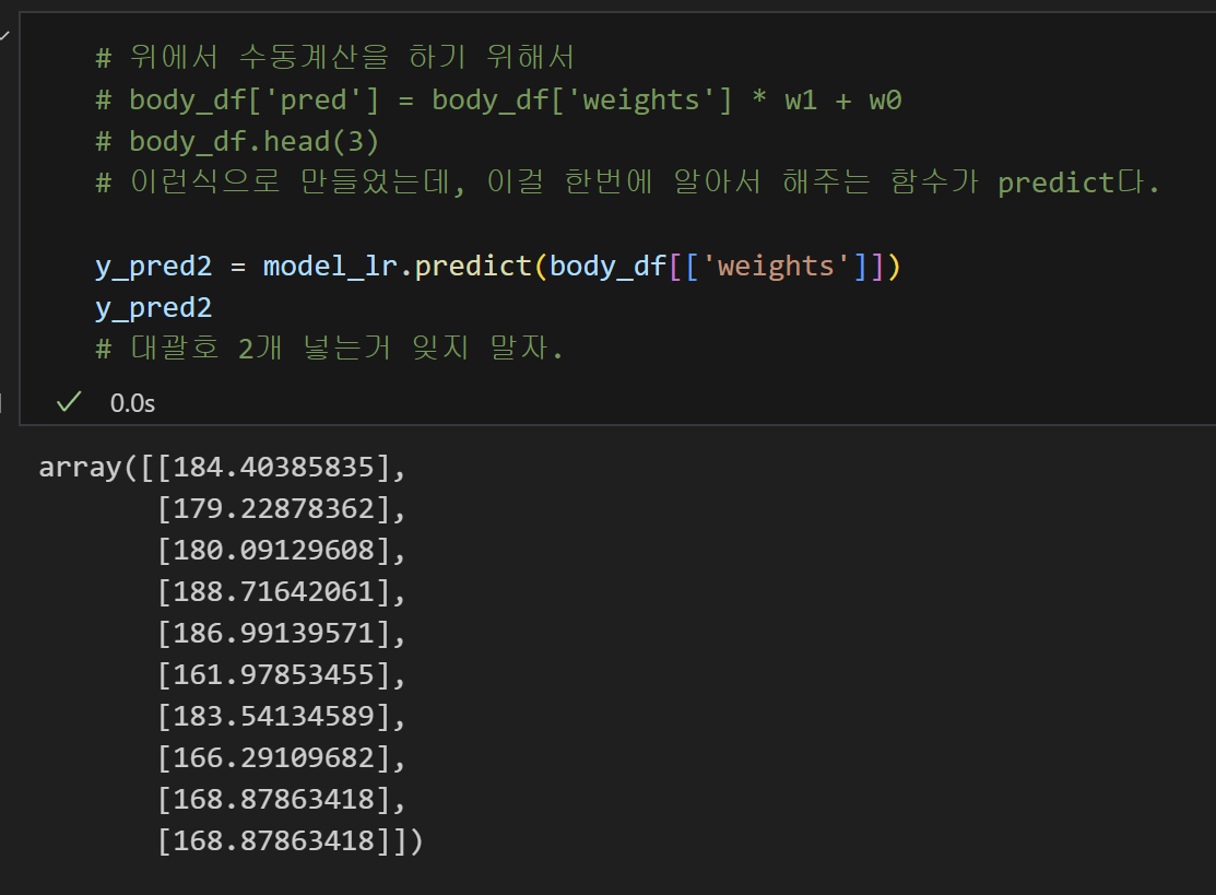
4-1) predict 함수를 활용하여 예측 컬럼 추가

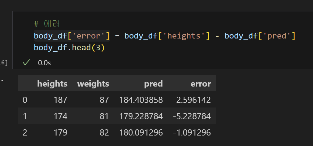
5) Error 값을 계산

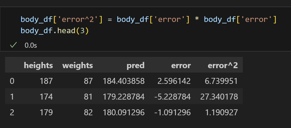
6) 양수로 만들기 위해서 제곱!

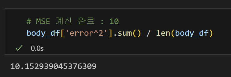
7) MSE 계산 완료!

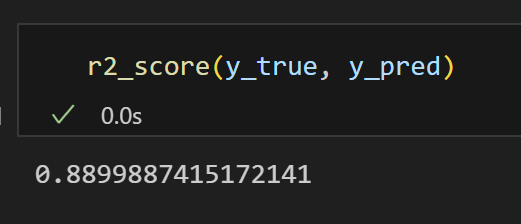
8) R Square 계산 완료!

= 88%의 설명력을 가지는 모델이다.

9) 산점도로 시각화

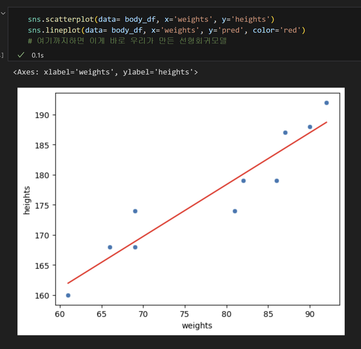
이렇게 하면 선형회귀 모델을 만들고, 평가하는 것 까지 했다!

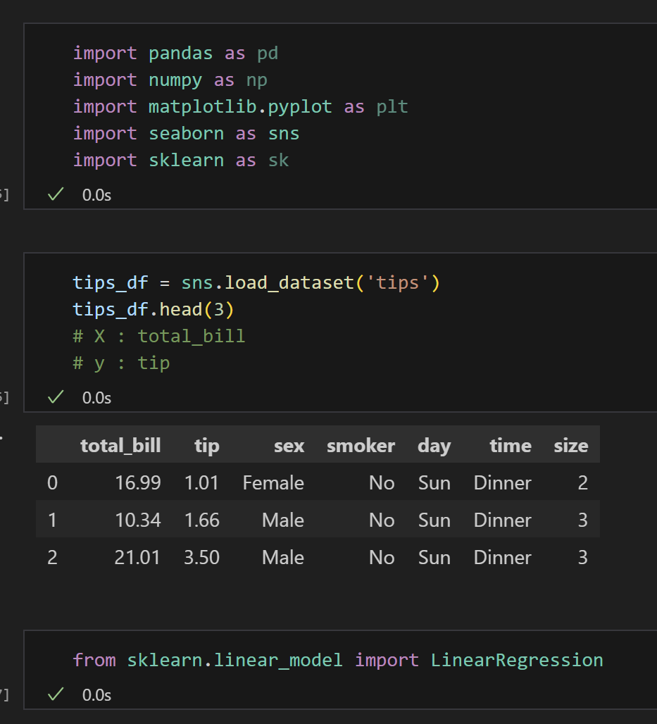
2. tips 데이터 실습

• 식당에서 파트타임으로 일하고 있는 머신이는 이번에는 tip 데이터를 가지고 적용해보기로 했다. 돈을 많이 벌고 싶었던 머신이는 전체 금액(X)를 알면 받을 수 있는 팁(Y)에 대한 회귀분석을 진행해 볼 예정이다.

1) 데이터 생성 및 라이브러리 설치

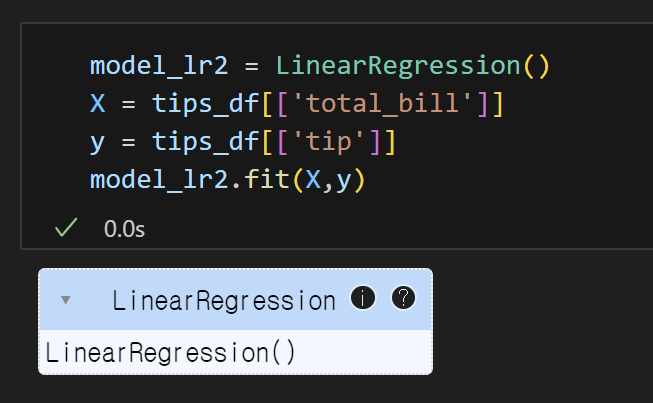
2) 선형회귀모델을 불러오고 데이터 훈련하기

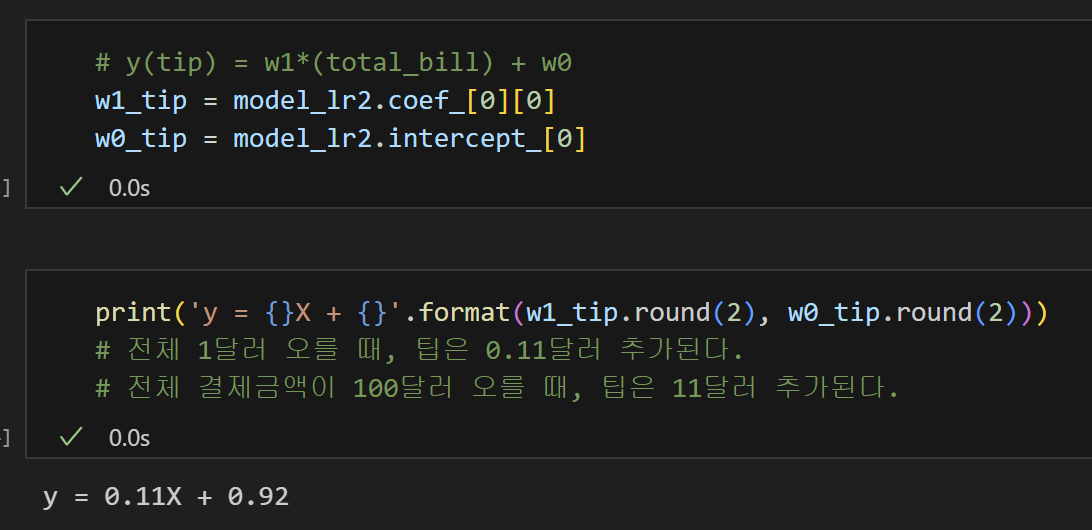
3) 가중치와 편향 구하기

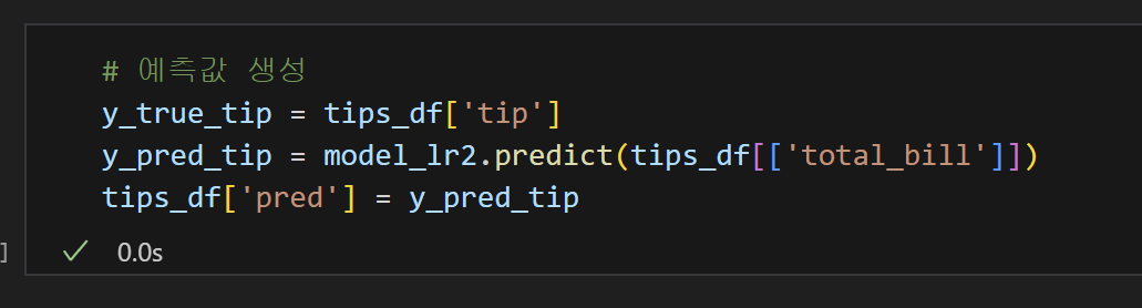
4) 예측 컬럼 만들기

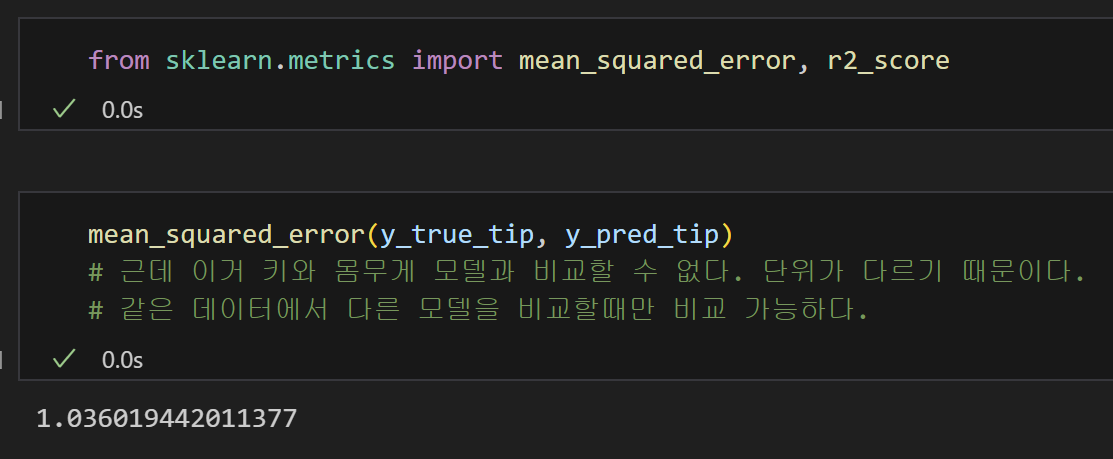
5) MSE 계산완료!

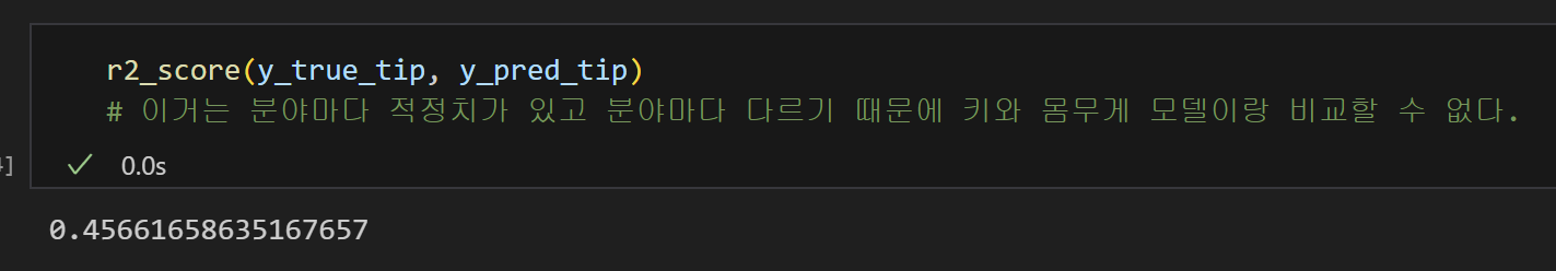
6) R Square 계산완료!

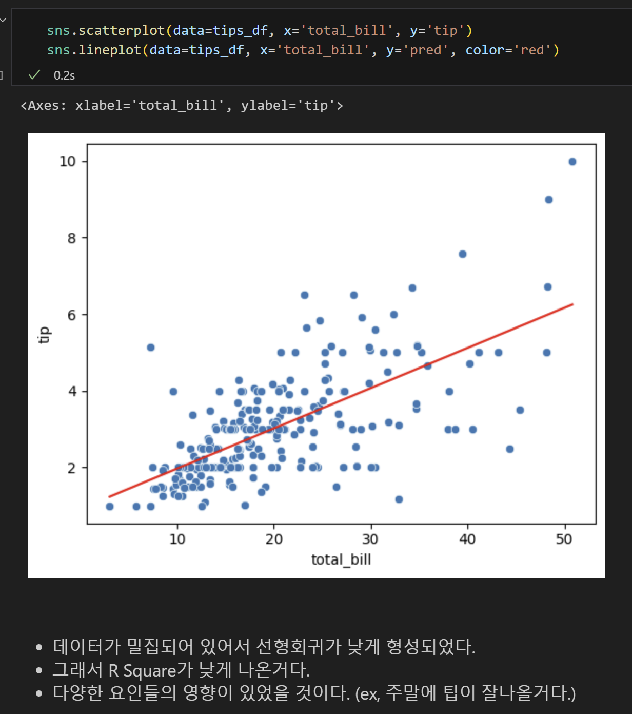
= 약 46%의 설명력을 가지는 모델이다.

• 근데 분야마다 적정치가 있기 때문에 판단할 수 없다.

7) 산점도 시각화