서론
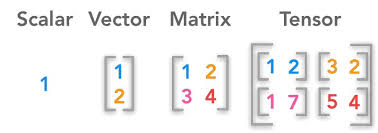
텐서(Tensor)는 배열(Array)이나 행렬(Matrix)과 매우 유사한 특수한 자료구조이다.
PyTorch에서는 텐서를 사용하여 모델의 입력과 출력뿐만 아니라 모델의 매개변수를 부호화(encode)한다.
Tensor
Tensor는 PyTorch의 핵심 데이터구조로서, NumPy의 다차원 배열과 유사한 형태로 데이터를 표현함
0-D Tensor
t = torch.tensor(36.5)
print('t =', t)
t = tensor(36.5000)
1-D Tensor
t = torch.tensor([175, 60, 81, 0.8, 0.9])
print('t =', t)
t = tensor([175.0000, 60.0000, 81.0000, 0.8000, 0.9000])
2-D Tensor
t = torch.tensor([[77, 114, 140, 191],
                  [39, 56, 46, 119],
                  [61, 29, 20, 33]])
print('t =', t)
t = tensor([[77, 114, 140, 191],
[ 39, 56, 46, 119],
[ 61, 29, 20, 33]])
3-D Tensor
t = torch.tensor([[[255, 0], [0, 255]],
				  [[0, 255], [0, 255]],
                  [[0, 0], [255, 0]]])
print('t =', t)
t = tensor([[[255, 0], [0, 255]],
[[0, 255], [0, 255]],
[[0, 0], [255, 0]]])
N-D Tensor
동일한 크기의 (N-1)-D Tensor들이 여러 개 쌓여 형성된 입체적인 배열 구조
데이터 타입
- 정수형 데이터 타입
- dtype = torch.uint8(8비트 부호 없는 정수)
- dtype = torch.int8(8비트 부호 있는 정수)
- dtype = torch.int16(16비트 부호 있는 정수)
- dtype = torch.int32(32비트 부호 있는 정수)
- dtype = torch.int64(64비트 부호 있는 정수)
- 실수형 데이터 타입(부동 소수점)
- dtype = torch.float32(32비트 부호 있는 실수)
- dtype = torch.float64(64비트 부호 있는 실수)
t = torch.tensor(-1, dtype = torch.int8)
print('t =', t)
print('t.dtype =', t.dtype)
t = tensor(-1, dtype=torch.int8)
t.dtype = torch.int8
t = torch.tensor(1, dtype = torch.float32)
print('t =', t)
print('t.dtype =', t.dtype)
t = tensor(1.)
t.dtype = torch.float32
타입 캐스팅
Tensor의 타입을 변경할 수 있음
t = torch.tensor([2, 3, 4], dtype = torch.int8)
t_ = t.float()
print('t_.dtype =', t_.dtype)
t_.dtype = torch.float32
기초 메서드
- min()
- Tensor의 모든 요소들 중 최소값을 계산하는 함수
- max()
- Tensor의 모든 요소들 중 최대값을 계산하는 함수
- sum()
- Tensor의 모든 요소들의 합을 계산하는 함수
- prod()
- Tensor의 모든 요소들의 곱을 계산하는 함수
- mean()
- Tensor의 모든 요소들의 평균을 계산하는 함수
- var()
- ensor의 모든 요소들의 표본분산을 계산하는 함수
- std()
- Tensor의 모든 요소들의 표본표준편차를 계산하는 함수
t = torch.tensor([[1, 2, 3],
                  [3, 4, 5]], dtype = torch.float)

print('torch.min(t) =', torch.min(t))
print('torch.max(t) =', torch.max(t))
print('torch.sum(t) =', torch.sum(t))
print('torch.prod(t) =', torch.prod(t))
print('torch.mean(t) =', torch.mean(t))
print('torch.var(t) =', torch.var(t))
print('torch.std(t) =', torch.std(t))
torch.min(t) = tensor(1.)
torch.max(t) = tensor(5.)
torch.sum(t) = tensor(18.)
torch.prod(t) = tensor(360.)
torch.mean(t) = tensor(3.)
torch.var(t) = tensor(2.)
torch.std(t) = tensor(1.4142)
특성 메서드
- dim()
- Tensor의 차원의 수를 확인하는 함수
- size()
- Tensor의 모양(크기)를 확인하는 함수
- shape()
- Tensor의 모양(크기)를 확인하는 함수
- numel()
- Tensor의 요소의 총 개수를 확인하는 함수
t = torch.tensor([[1, 2, 3],
                  [3, 4, 5]], dtype = torch.float)

print('t.dim() =', t.dim())
print('t.size() =', t.size())
print('t.shape() =', t.shape())
print('t.numel() =', t.numel())
t.dim() = 2
t.size() = torch.Size([2, 3])
t.shape = torch.Size([2, 3])
t.numel() = 6
생성
특정 값으로 초기화된 Tensor
- zeros()
- 모든 요소들의 값이 0인 Tensor 생성
- zeros_like(s)
- s와 shape가 일치하며 모든 요소들의 값이 0인 Tensor 생성
- ones()
- 모든 요소들의 값이 1인 Tensor 생성
- ones_like(s)
- s와 shape가 일치하며 모든 요소들의 값이 1인 Tensor 생성
t = torch.zeros([2, 3])
print('t =', t)
t = tensor([[0., 0., 0.],
[0., 0., 0.]])
t = torch.ones([3, 2])
print('t =', t)
t = tensor([[1., 1.],
[1., 1.],
[1., 1.]])
난수로 초기화된 Tensor
- rand()
- 연속균등분포 난수 값을 요소로 갖는 Tensor 생성
- randn()
- 표준정규분포 난수 값을 요소로 갖는 Tensor 생성
t = torch.rand([2, 3])
print('t =', t)
t = tensor([[0.4605, 0.0048, 0.3104],
[0.9032, 0.9522, 0.2036]])
t = torch.randn([2, 3])
print('t =', t)
t = tensor([[ 0.7108, -0.3084, 0.5309],
[ 0.0119, -0.7204, -0.9224]])
지정 범위 내 값으로 초기화된 Tensor
- arange(start, end, step)
- start 값부터 end 값 직전까지 step씩 더한 값을 요소로 갖는 Tensor 생성
- Tensor의 요소 중 float 자료형이 포함된다면 t.dtype = float
- Tensor의 요소 중 float 자료형이 포함되지 않는다면 t.dtype = int
t = torch.arange(start = 1, end = 11, step = 2)
# t = torch.arange(1, 11, 2)
print('t =', t)
print('t.dtype =', t.dtype)
t = tensor([1, 3, 5, 7, 9])
t.dtype = torch.int64
t = torch.arange(start = 1, end = 4, step = 0.5)
# t = torch.arange(1, 4, 0.5)
print('t =', t)
print('t.dtype =', t.dtype)
t = tensor([1.0000, 1.5000, 2.0000, 2.5000, 3.0000, 3.5000])
t.dtype = torch.float32
초기화되지 않은 Tensor
- empty()
- 초기화되지 않은 Tensor 생성
- fill_()
- 초기화 되지 않은 Tensor의 값 수정
- 메모지 주소 변경 X
- 성능 향상, 메모리 사용 최적화
- Tensor 생성 후 곧바로 다른 값으로 덮어씌울 예정이라면 초기 값 설정이 불필요한 자원 소모임
t = torch.empty(5)
print('t =', t)
t = tensor([-1.5359e+10, 4.5846e-41, -1.5359e+10, 4.5846e-41, 4.4842e-44])
torch.fill_(t, 3.0)
print('t =', t)
t = tensor([3., 3., 3., 3., 3.])
t = torch.empty([2, 3])
print('t =', t)
t = tensor([[-1.5359e+10, 4.5846e-41, -1.3635e-17],
[ 3.1361e-41, 4.4842e-44, 0.0000e+00]])
torch.fill_(t, 3.0)
print('t =', t)
t = tensor([[3., 3., 3.],
[3., 3., 3.]])
list, Numpy 기반 Tensor
- tensor()
- list 기반 Tensor 생성
- from_numpy()
- Numpy 기반 Tensor 생성
s = [1, 2, 3, 4, 5, 6]
t = torch.tensor(s)
print('t =', t)
t = tensor([1, 2, 3, 4, 5, 6])
import numpy as np

s = np.array([[0, 1],
              [2, 3]])
t = torch.from_numpy(s)
print('t =', t)
t = tensor([[0, 1],
[2, 3]])
CPU Tensor
- IntTensor()
- 정수형 CPU Tensor 생성
- FloatTensor()
- 실수형 CPU Tensor 생성
s = [1, 2, 3, 4, 5]
t = torch.IntTensor(s)
print('t =', t)
t = tensor([1, 2, 3, 4, 5], dtype=torch.int32)
import numpy as np

s = [1, 2, 3, 4, 5]
t = torch.FloatTensor(s)
print('t =', t)
t = tensor([1., 2., 3., 4., 5.])
CUDA Tensor
- GPU(Graphics Processing Unit): 그래픽 처리 장치
- 현재 AI 연구 및 개발에 있어 대규모 데이터 처리와 복잡한 계산에 사용
- 병렬 처리 능력: GPU는 수천 개의 작은 코어를 가지고 있어 대량의 연산 동시 수행 가능
- cuda.is_available()
- GPU를 사용할 수 있는 환경인지 확인
- cuda.get_device_name()
- GPU 디바이스 이름 확인
- cuda.device_count()
- 사용 가능한 GPU 개수 확인
- tensor.cuda()
- Tensor를 GPU에 할당
- tensor.cpu()
- GPU에 할당된 Tensor를 CPU Tensor로 변환
t = torch.tensor([1, 2, 3])
print(t.device)
device(type='cpu')
print(torch.cuda.is_available())True
print(torch.cuda.get_device_name(device=0))'Tesla T4'
print(torch.cuda.device_count())1
t = torch.tensor([1, 2, 3, 4, 5]).cuda()
# t = torch.tensor([1, 2, 3, 4, 5]).to(device = 'cuda')
print('t_gpu = ', t)
t_gpu = tensor([1, 2, 3, 4, 5], device='cuda:0')
t = torch.tensor([1, 2, 3, 4, 5]).cpu()
# t = torch.tensor([1, 2, 3, 4, 5]).to(device = 'cpu')
print('t_gpu = ', t)
t_cpu = tensor([1, 2, 3, 4, 5])
# 실제 사용 예시
device = torch.device('cuda' if torch.cuda.is_available() else 'cpu')
t = t.to(device)
Shape 참조
- zeros_like(s)
- s와 shape가 동일하며 모든 요소들의 값이 0인 Tensor 생성
- ones_like(s)
- s와 shape가 동일하며 모든 요소들의 값이 1인 Tensor 생성
- rand_like(s)
- s와 shape가 동일하며 연속균등분포 난수 값을 요소로 갖는 Tensor 생성
- randn_like(s)
- s와 shape가 동일하며 표준정규분포 난수 값을 요소로 갖는 Tensor 생성
s = torch.ones([2, 3])
t = torch.zeros_like(s)
print('t =', t)
t = tensor([[0., 0., 0.],
[0., 0., 0.]])
s = torch.zeros([2, 3])
t = torch.ones_like(s)
print('t =', t)
t = tensor([[1., 1., 1.],
[1., 1., 1.]])
s = torch.zeros([2, 3])
t = torch.rand_like(s)
print('t =', t)
t = tensor([[0.6924, 0.1830, 0.2530],
[0.4801, 0.5337, 0.7290]])
s = torch.zeros([2, 3])
t = torch.randn_like(s)
print('t =', t)
t = tensor([[-1.0576, 1.4039, 0.8849],
[-0.7208, 0.3792, 0.4855]])
복제
- clone()
- Tensor 복제, 계산 그래프 분리 X
- detach()
- Tensor 복제, 계산 그래프 분리 O
s = torch.tensor([1, 2, 3, 4, 5, 6])
t = s.clone()
print('t =', t)
t = tensor([1, 2, 3, 4, 5, 6])
s = torch.tensor([1, 2, 3, 4, 5, 6])
t = s.detach()
print('t =', t)
t = tensor([1, 2, 3, 4, 5, 6])
인덱싱
- Indexing
- Tensor의 특정 요소에 접근
- 음수 값도 Index로 사용 가능
t = torch.tensor([10, 20, 30, 40, 50, 60])
print('t[0] =', t[0])
t[0] = tensor(10)
t = torch.tensor([10, 20, 30, 40, 50, 60])
print('t[-2] =', t[-2])
t[-2] = tensor(50)
t = torch.tensor([[10, 20, 30],
                  [40, 50, 60]])
print('t[1, 2] = ', t[1, 2])
# print('t[1, 2] = ', t[1][2])
t[1, 2] = tensor(60)
슬라이싱
- Slicing
- 부분집합을 선택하여 sub Tensor 생성
- 리스트의 Slicing과 유사
t = torch.tensor([10, 20, 30, 40, 50, 60])
print('t[1:4] =', t[1:4])
t[1:4] = tensor([20, 30, 40])
t = torch.tensor([[10, 20, 30],
                  [40, 50, 60]])
print('t[1, 2] = ', t[1, 2])
t[:, 1:] = tensor([[20, 30],
[50, 60]])
차원 재구성
Shape 변경
- view()
- Tensor의 Shape 변경
- Tensor의 요소들이 메모리에 연속적으로 할당된 경우 사용 가능
- Tensor의 요소들은 기본적으로 메모리에 연속적으로 할당됨
- Slicing 이후 Tensor의 요소들이 비연속적으로 할당될 수 있음
- is_contiguous() 메서드를 통해 연속적인지 확인 가능
- t = t.contiguous() 메서드를 통해 연속적으로 재할당 가능
- N개의 차원 중 N - 1개 입력 시 나머지 하나의 차원에 해당하는 인자로 -1 사용 가능
- reshape()
- Tensor의 Shape 변경
- Tensor의 요소들이 메모리에 비연속적으로 할당된 경우에도 사용 가능
- 안전, 유연 But 성능 저하
s = torch.tensor([[0, 1, 2],
                  [3, 4, 5]])
t = s[:, :2]

if not t.is_contiguous():
	t = t.contiguous()
    print("Reallocation is done.")

t = t.view(1, -1)
print('t =', t)
Reallocation is done.
t = tensor([[0, 1, 3, 4]])
t = torch.arange(12)
t = t.reshape(2, -1)
print('t =', t)
t = tensor([[ 0, 1, 2, 3, 4, 5],
[ 6, 7, 8, 9, 10, 11]])
평탄화
- flatten(start_dim, end_dim)
- start_dim 부터 end_dim까지 평탄화
- end_dim 인자가 없다면 start_dim부터 tensor의 마지막 dim까지 평탄화
s = torch.zeros(3, 2, 2)
t = s.flatten(0)
print('t.shape =', t.shape)
t.shape = torch.Size([12])
s = torch.zeros(3, 2, 2)
t = s.flatten(1)
print('t.shape =', t.shape)
t.shape = torch.Size([3, 4])
s = torch.zeros(3, 2, 2)
t = s.flatten(2)
print('t.shape =', t.shape)
t.shape = torch.Size([3, 2, 2])
s = torch.zeros(3, 2, 2)
t = s.flatten(0, 1)
print('t.shape =', t.shape)
t.shape = torch.Size([6, 2])
Transpose
- transpose(dim_1, dim_2)
- dim_1 과 dim_2 전치
s = torch.tensor([[0, 1, 2],
                 [3, 4, 5]])
t = s.transpose(0, 1)
print('t =', t)
t = tensor([[0, 3],
[1, 4],
[2, 5]])
s = torch.tensor([[[0, 1],
                  [2, 3],
                  [4, 5]],

                 [[6, 7],
                  [8, 9],
                  [10, 11]],

                 [[12, 13],
                  [14, 15],
                  [16, 17]]])
t = s.transpose(1, 2)
print('t =', t)
t = tensor([[[ 0, 2, 4], [ 1, 3, 5]],
[[ 6, 8, 10], [ 7, 9, 11]],
[[12, 14, 16], [13, 15, 17]]])
차원 축소
- squeeze()
- dim이 1인 차원 삭제
square bracket('[', ']')을 삭제할 수 있는 경우 squeeze()함수로 삭제한다 생각
s = torch.zeros(1, 3, 4)
t = s.squeeze()
print('s =', s, '\n')
print('t =', t, '\n')
print('t.shape =', t.shape)
s = tensor([[[0., 0., 0., 0.],
[0., 0., 0., 0.],
[0., 0., 0., 0.]]])
t = tensor([[0., 0., 0., 0.],
[0., 0., 0., 0.],
[0., 0., 0., 0.]])
t.shape = torch.Size([3, 4])
차원 확장
- unsqueeze(dim)
- dim 차원 추가
square bracket('[', ']')을 unsqueeze()함수로 추가한다 생각
s = torch.zeros(3, 4)
t = s.unsqueeze(dim=1)
print('s =', s, '\n')
print('t =', t, '\n')
print('t.shape =', t.shape)
s = tensor([[0., 0., 0., 0.],
[0., 0., 0., 0.],
[0., 0., 0., 0.]])
t = tensor([[[0., 0., 0., 0.]],
[[0., 0., 0., 0.]],
[[0., 0., 0., 0.]]])
t.shape = torch.Size([3, 1, 4])
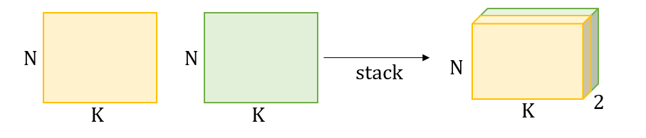
결합
- stack(tuple, dim)
- 여러 tensor를 dim 방향으로 쌓여 새로운 tensor 생성
- 새로운 차원이 생성
- tensor들을 tuple 형식으로 묶어 인자로 넘겨야 함
- dim 값이 없다면 dim = 0
- cat(tuple, dim)
- 여러 tensor를 dim 방향으로 연결하여 새로운 tensor 생성
- 기존 차원이 유지
- tensor들을 tuple 형식으로 묶어 인자로 넘겨야 함
- dim 값이 없다면 dim = 0
- dim 기준 shape 값이 일치하지 않는다면 에러 발생
출처: https://sanghyu.tistory.com/85
red_channel = torch.tensor([[255, 0],
                            [0, 255]])
green_channel = torch.tensor([[0, 255],
                              [0, 255]])
blue_channel = torch.tensor([[0, 0],
                             [255, 0]])

t = torch.stack((red_channel, green_channel, blue_channel), dim = 0)
print('t =', t)
print('t.shape = ', t.shape)
t = tensor([[[255, 0],
[0, 255]],
[[ 0, 255],
[0, 255]],
[[0, 0],
[255, 0]]])
t.shape = torch.Size([3, 2, 2])
u = torch.tensor([[0, 1],
                  [2, 3]])
v = torch.tensor([[4, 5]])
t = torch.cat((u, v))
print('t =', t)
print('t.shape =', t.shape)
t = tensor([[0, 1],
[2, 3],
[4, 5]])
t.shape = torch.Size([3, 2])
u = torch.tensor([[0, 1],
                  [2, 3]])
v = torch.tensor([[4, 5]])
t = torch.cat((u, v), dim=1)
print('t =', t)
print('t.shape =', t.shape)
Error
u = torch.tensor([[0, 1],
                  [2, 3]])
v = torch.tensor([[4, 5]])
t = torch.cat((u, v.view(2, 1)), dim=1)
print('t =', t)
print('t.shape =', t.shape)
t = tensor([[0, 1, 4],
[2, 3, 5]])
t.shape = torch.Size([2, 3])
크기 확장
- expand(dim_1_size, dim_2_size)
- 크기가 1인 차원의 크기 확장
- shape: (dim_1_size * dim_2_size)
- 크기가 1인 차원이 존재해야 사용 가능
- repeat(dim_1_times, dim_2_times)
- 차원의 크기 확장
- shape: ((dim_1_size * dim_1_times) * (dim_2_size * dim_2_times))
t = torch.tensor([[1, 2, 3]])
t = t.expand(4, 3)

print('t =', t)
print('t.shape =', t.shape)
t = tensor([[1, 2, 3],
[1, 2, 3],
[1, 2, 3],
[1, 2, 3]])
t.shape = torch.Size([4, 3])
t = torch. tensor([[1, 2],
                   [3, 4]])
t = t.repeat(2, 3)
print('t =', t)
print('t.shape =', t.shape)
t = tensor([[1, 2, 1, 2, 1, 2],
[3, 4, 3, 4, 3, 4],
[1, 2, 1, 2, 1, 2],
[3, 4, 3, 4, 3, 4]])
t.shape = torch.Size([4, 6])
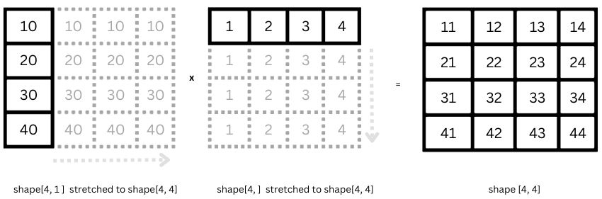
기초 연산
BroadCasting
Tensor 연산 시 shape가 일치하지 않는다면 연산이 가능하도록 각 Tensor를 확장
출처: https://www.machinelearningnuggets.com/tensorflow-tensors-what-are-tensors-understanding-the-basics-creating-and-working-with-tensors/
Inplace 방식
- 추가적인 메모리 할당 없이 tensor_1에 연산 결과를 덮어 씌움
- Autograd와의 호환성 측면에서 문제를 일으킬 수 있음
u = torch.tensor([[1, 2],
                  [3, 4]])
v = torch.tensor([[1, 3],
                  [5, 7]])

print('u+v =', u.add_(v))
u+v = tensor([[ 2, 5],
[8, 11]])
산술 연산
- add(tensor_1, tensor_2)
- tensor의 덧셈
- sub(tensor_1, tensor_2)
- tensor의 뺄셈
- mul(tensor_1, tensor_2)
- tensor의 곱셈
- div(tensor_1, tensor_2)
- tensor의 나눗셈
- pow(tensor, scalar)
- tensor의 거듭제곱
- pow(t, n): t의 n 거듭제곱
- pow(t, 1/n): t의 n 거듭제곱근
u = torch.tensor([[1, 2],
                  [4, 5]])
v = torch.tensor([1, 3])
print('u+v =', torch.add(u, v))
u+v = tensor([[2, 5],
[5, 8]])
u = torch.tensor([[1, 2],
                  [4, 5]])
v = torch.tensor([1, 3])
print('u+v =', torch.sub(u, v))
u+v = tensor([[0, -1],
[3, 2]])
u = torch.tensor([[1, 2],
                  [4, 5]])
v = torch.tensor([1, 3])
print('u+v =', torch.mul(u, v))
u+v = tensor([[1, 6],
[4, 15]])
u = torch.tensor([[18, 9],
                  [10, 4]])
v = torch.tensor([[6, 3],
                  [5, 2]])
print('u+v =', torch.div(u, v))
u+v = tensor([[3., 3.],
[2., 2.]])
t = torch.tensor([[1, 2],
                  [3, 4]])
print('t^2 =', torch.pow(t, 2))
print('t^3 =', torch.pow(t, 3))
t^2 = tensor([[ 1, 4],
[ 9, 16]])
t^3 = tensor([[ 1, 8],
[27, 64]])
비교 연산
- eq(tensor_1, tensor_2)
- equal to
- result[i] = (tensor_1[i] == tensor_2[i])
- ne(tensor_1, tensor_2)
- not equal to
- result[i] = (tensor_1[i] != tensor_2[i])
- gt(tensor_1, tensor_2)
- greater than
- result[i] = (tensor_1[i] > tensor_2[i])
- ge(tensor_1, tensor_2)
- greater than or eqaul to
- result[i] = (tensor_1[i] >= tensor_2[i])
- lt(tensor_1, tensor_2)
- less than
- result[i] = (tensor_1[i] < tensor_2[i])
- le(tensor_1, tensor_2)
- less than or eqaul to
- result[i] = (tensor_1[i] <= tensor_2[i])
u = torch.tensor([1, 3, 5, 7])
v = torch.tensor([2, 3, 5, 7])
print('u == v :', torch.eq(u, v))
print('u != v :', torch.ne(u, v))
print('u > v :', torch.gt(u, v))
print('u >= v :', torch.ge(u, v))
print('u < v :', torch.lt(u, v))
print('u <= v :', torch.le(u, v))
u == v : tensor([False, True, True, True])
u != v : tensor([ True, False, False, False])
u > v : tensor([False, False, False, False])
u >= v : tensor([False, True, True, True])
u < v : tensor([ True, False, False, False])
u <= v : tensor([True, True, True, True])
논리 연산
- logical_and(tensor_1, tensor_2)
- result[i] = (tensor_1[i] and tensor_2[i])
- logical_or(tensor_1, tensor_2)
- result[i] = (tensor_1[i] or tensor_2[i])
- logical_xor(tensor_1, tensor_2)
- result[i] = (tensor_1[i] xor tensor_2[i])
u = torch.tensor([True, True, False, False])
v = torch.tensor([True, False, True, False])
print('and(u, v) =', torch.logical_and(u, v))
print('or(u, v) =', torch.logical_or(u, v))
print('xor(u, v) =', torch.logical_xor(u, v))
and(u, v) = tensor([ True, False, False, False])
or(u, v) = tensor([ True, True, True, False])
xor(u, v) = tensor([False, True, True, False])
Norm
L1 Norm (맨해튼 Norm)
t = torch.tensor([4, 3], dtype=torch.float32)
L1_norm = torch.norm(t, p=1)
print(f'L1 Norm of a: {L1_norm}')
L1 Norm of a: 7.0
L2 Norm (유클리드 Norm)
t = torch.tensor([4, 3], dtype=torch.float32)
L2_norm = torch.norm(t, p=2)
print(f'L2 Norm of a: {L2_norm}')
L2 Norm of a: 5.0
유사도
두 1-D Tensor가 얼마나 유사한지에 대한 측정값
맨해튼 유사도
u = torch.tensor([1, 0, 2], dtype=torch.float32)
v = torch.tensor([0, 1, 2], dtype=torch.float32)

manhattan_distance = torch.norm(u - v, p = 1)
manhattan_similarity = 1 / (1 + manhattan_distance)

print(f'Manhattan Distance: {manhattan_distance}')
print(f'Manhattan Similarity: {manhattan_similarity}')
Manhattan Distance: 2.0
Manhattan Similarity: 0.3333333432674408
유클리드 유사도
u = torch.tensor([1, 0, 2], dtype=torch.float32)
v = torch.tensor([0, 1, 2], dtype=torch.float32)

euclidean_distance = torch.norm(u - v, p = 2)
euclidean_similarity = 1 / (1 + euclidean_distance)

print(f'Euclidean Distance: {euclidean_distance}')
print(f'Euclidean Similarity: {euclidean_similarity}')
Euclidean Distance: 1.4142135381698608
Euclidean Similarity: 0.41421353816986084
코사인 유사도
u = torch.tensor([1, 0, 2], dtype=torch.float32)
v = torch.tensor([0, 1, 2], dtype=torch.float32)

dot_product = torch.dot(u, v)
cosine_similarity = torch.dot(u, v) / (torch.norm(u, p = 2) * torch.norm(v, p = 2))

print(f'Cosine Similarity: {cosine_similarity}')
Cosine Similarity: 0.800000011920929
2-D 곱셈 연산
- matmul(tensor_1, tensor_2)
- mm(tensor_1, tensor_2) 혹은 tensor_1 @ tensor_2로 대체 가능
u = torch.tensor([[1, 1, 3],
                  [4, 5, 6],
                  [7, 8, 9]])
v = torch.tensor([[1, 0],
                  [1, -1],
                  [2, 1]])

t = torch.matmul(u, v)
# t = torch.mm(u, v)
# t = u @ v
print('t =', t)
t = tensor([[ 8, 2],
[21, 1],
[33, 1]])
대칭
- flip(tensor, list)
- tensor를 list 내의 dim 기준으로 대칭
t = torch.tensor([[[1, 2, 3],
                  [4, 5, 6]],
                  [[3, 2, 4],
                   [5, 2, 1]]])
symmetric_t = torch.flip(t, [0])
print('symmetric_t =',symmetric_t)
symmetric_t = tensor([[[3, 2, 4],
[5, 2, 1]],
[[1, 2, 3],
[4, 5, 6]]])
t = torch.tensor([[[1, 2, 3],
                  [4, 5, 6]],
                  [[3, 2, 4],
                   [5, 2, 1]]])
symmetric_t = torch.flip(t, [1])
print('symmetric_t =',symmetric_t)
symmetric_t = tensor([[[4, 5, 6],
[1, 2, 3]],
[[5, 2, 1],
[3, 2, 4]]])
t = torch.tensor([[[1, 2, 3],
                  [4, 5, 6]],
                  [[3, 2, 4],
                   [5, 2, 1]]])
symmetric_t = torch.flip(t, [0, 1])
print('symmetric_t =',symmetric_t)
symmetric_t = tensor([[[5, 2, 1],
[3, 2, 4]],
[[4, 5, 6],
[1, 2, 3]]])
결론
PyTorch의 Tensor는 딥러닝과 머신러닝에서 데이터 처리를 위한 필수적인 도구이다.
다양한 차원에서의 표현과 강력한 연산 기능을 통해, 연구자와 개발자들은 복잡한 모델을 쉽게 구현하고 학습시킬 수 있다.
Tensor는 단순한 데이터 구조 이상의 의미를 가지며, GPU 가속을 통한 고속 연산과 자동 미분 기능으로 신경망 학습의 효율성을 높여준다.
본 글에서 설명한 다양한 Tensor의 유형과 연산, 초기화 방법, 데이터 타입 변환 및 변형 기법들은 PyTorch를 활용하는 데 있어 기초적인 이해를 돕는다.
이를 통해 사용자는 자신만의 모델을 설계하고 최적화하며, 더 나아가 데이터 과학 및 인공지능 분야의 다양한 문제를 해결할 수 있는 능력을 갖추게 된다.
