Binary Classification

AAiss·2024년 8월 12일

AI Basics

목록 보기

6/12

서론

이진 분류는 머신러닝에서 가장 기본적이며 널리 사용되는 문제 유형 중 하나로, 주어진 입력 데이터가 두 개의 클래스 중 하나에 속하는지를 판단하는 과정이다.

로지스틱 회귀는 이진 분류 문제를 해결하기 위한 대표적인 기법으로, 확률적 접근 방식을 통해 클래스 레이블을 예측한다.

본 포스팅에서는 이진 분류의 개념부터 시작하여, 데이터 전처리, 모델 학습, 그리고 평가 방법까지 단계별로 살펴보겠다.

로지스틱 회귀

트레이닝 데이터의 특성과 분포를 바탕으로 데이터 구분을 위한 최적의 선형 결정 경계 탐색

시그모이드 함수를 통해 선형 결정 경계를 비선형 결정 경계로 변환

이를 바탕으로 모델 학습, 테스트 데이터의 결과를 레이블로 예측

데이터 전처리

특징 변수( $x$ ) - PetalLengthCm

목표 변수( $t$ ) - Species

사용 데이터셋: Iris Dataset
저작권 정보: CC0 1.0 Universal

데이터 로드

# Donwload dataset from kaggle
!kaggle datasets download -d uciml/iris
# unzip zip file
!unzip iris.zip

import pandas as pd

df = pd.read_csv("Iris.csv", sep = ",", header = 0)[["PetalLengthCm", "Species"]]
filtered_df = df[df['Species'].isin(['Iris-setosa', 'Iris-versicolor'])]  # 필요 데이터만 추출

목표 변수를 이산형 레이블로 매핑

filtered_df.loc[:, 'Species'] = filtered_df['Species'].map({'Iris-setosa': 0, 'Iris-versicolor': 1})

특징 변수와 목표 변수 분리

x = filtered_df[['PetalLengthCm']].values
t = filtered_df['Species'].values.astype(int)

데이터 분할

트레이닝 데이터: 모델 학습에 사용되는 데이터 (가중치, 바이어스 최적화)

테스트 데이터: 최종 모델의 성능 평가에 사용되는 데이터

검증 데이터: 모델의 학습 과정 중 사용되는 데이터 (모델의 에폭마다 과적합 확인)

from sklearn.model_selection import train_test_split

x_train, x_test, t_train, t_test = train_test_split(x, t, test_size=0.2, random_state=42)

데이터 표준화

from sklearn.preprocessing import StandardScaler

scaler = StandardScaler()
x_train = scaler.fit_transform(x_train)
x_test = scaler.transform(x_test)

Tensor로 변환

# 배치 처리 및 일관된 데이터 형태를 위해 목표 변수를 2차원 Tensor로 변환
x_train = torch.tensor(x_train, dtype=torch.float32)
x_test = torch.tensor(x_test, dtype=torch.float32)
t_train = torch.tensor(t_train, dtype=torch.float32).unsqueeze(1)
t_test = torch.tensor(t_test, dtype=torch.float32).unsqueeze(1)

배치(Batch)

ML/DL에서 데이터를 처리하는 묶음의 단위

미니배치 경사하강법

확률적 경사하강법은 계산이 빠르고 메모리 측면에서 효율적

하지만, 계산 과정에서 노이즈가 많고 학습 과정이 불안정

경사하강법과 확률적 경사하강법의 단점을 보완한 알고리즘

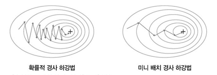출처: 서지영(2022). 딥러닝 파이토치 교과서. 서울; (주) 도서출판 길벗.

from torch.utils.data import Dataset, DataLoader

class IrisDataset(Dataset):   # CustomDataset 클래스
    def __init__(self, features, labels):
        self.features = features  # 특징 변수
        self.labels = labels  # 목표 변수

    def __len__(self):
        return len(self.features)

    def __getitem__(self, idx):
        return self.features[idx], self.labels[idx]

train_dataset = IrisDataset(x_train, t_train)
test_dataset = IrisDataset(x_test, t_test)

batch_size = 4
# 모델 훈련 시 데이터 순서에 따른 편향을 줄이기 위해 shuffle
train_loader = DataLoader(train_dataset, batch_size=batch_size, shuffle=True)
# 모델 성능 평가 시 데이터 순서 유지
test_loader = DataLoader(test_dataset, batch_size=batch_size, shuffle=False)

모델 학습

트레이닝 데이터의 특성과 분포를 바탕으로 데이터를 잘 구분할 수 있는 선형 결정 경계(직선) 탐색

직선: $z = wx + b$

최적의 $w$ (가중치)와 $b$ (바이어스) 탐색

시그모이드 함수를 통해 선형 결정 경계를 비선형 결정 경계(최적의 경계)로 변환

경계: $y = Sigmoid(z)$

이를 바탕으로 모델 학습, 테스트 데이터의 결과를 레이블로 예측

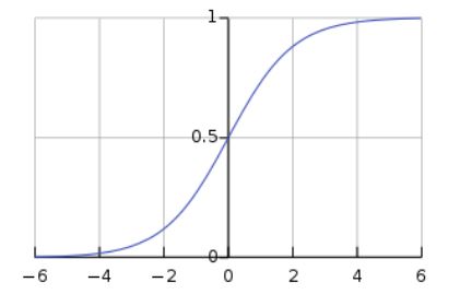
시그모이드 함수

비선형 함수

입력 값을 0과 1사이의 값으로 변환

$y = Sigmoid(z) = \frac{1}{1 + exp(-z)}$

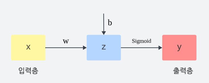
이진 분류 모델 (by 신경망)

입력층: 특징 변수들( $x$ )

출력층: 예측 변수( $y$ )

import torch.nn as nn

class BinaryClassificationModel(nn.Module):
    def __init__(self):
        super(BinaryClassificationModel, self).__init__()
        self.layer_1 = nn.Linear(1, 1)  # 입력 차원과 출력 차원을 1로 설정
        self.sigmoid = nn.Sigmoid()

    def forward(self, x):
        z = self.layer_1(x)
        y = self.sigmoid(z)
        return y
        
model = BinaryClassificationModel()

손실함수

BCE (Binary Cross Entropy)

이진 분류 문제에서 모델의 예측 변수와 목표 변수 간의 차이를 측정하기 위해 사용되는 손실 함수

$Loss\ Function = -\displaystyle\sum_{i=1}^{n}[t_i\log{y_i} + (1 - t_i)\log(1-y_i)]$

nn.BCELoss()

BCE 손실함수

import torch.optim as optim

loss_function = nn.BCELoss()
optimizer = optim.SGD(model.parameters(), lr=0.01)

num_epochs = 500
loss_list = []
for epoch in range(num_epochs):
    model.train()
    epoch_loss = 0
    for batch_features, batch_labels in train_loader:
        optimizer.zero_grad()
        outputs = model(batch_features)
        loss = loss_function(outputs, batch_labels)
        loss.backward()
        optimizer.step()
        epoch_loss += loss.item()

    loss_list.append(epoch_loss / len(train_loader))

    if (epoch+1) % 100 == 0:
        print(f'Epoch [{epoch+1}/{num_epochs}], Loss: {loss.item()}')

import matplotlib.pyplot as plt

plt.figure()
plt.plot(loss_list, label='Train Loss')
plt.xlabel('Epochs')
plt.ylabel('Loss')
plt.legend()
plt.grid(True)
plt.title('Loss Trend')
plt.show()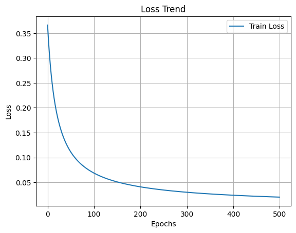

테스트

학습된 모델을 통해 테스트 데이터의 결과 예측

import numpy as np

model.eval()
with torch.no_grad():
    predictions = model(x_test)
    predicted_labels = (predictions > 0.5).float()

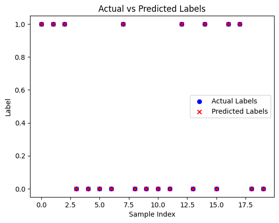
# 예측 결과와 실제 라벨을 출력하는 코드 표현 실습

actual_labels = t_test.numpy()
predicted_labels = predicted_labels.numpy()

print("Predictions:", predicted_labels.flatten())
print("Actual Labels:", actual_labels.flatten())

Predictions: [1. 1. 1. 0. 0. 0. 0. 1. 0. 0. 0. 0. 1. 0. 1. 0. 1. 1. 0. 0.]
Actual Labels: [1. 1. 1. 0. 0. 0. 0. 1. 0. 0. 0. 0. 1. 0. 1. 0. 1. 1. 0. 0.]

plt.figure()
plt.scatter(range(len(actual_labels)), actual_labels, color='blue', label='Actual Labels')
plt.scatter(range(len(predicted_labels)), predicted_labels, color='red', marker='x', label='Predicted Labels')
plt.xlabel('Sample Index')
plt.ylabel('Label')
plt.legend()
plt.title('Actual vs Predicted Labels')
plt.show()