SVM과 Decision Tree 실습
47일차에 사용 했었던 [비행 경험 만족도 데이터] 를 사용해서 실습해 볼 예정이다.
전처리 까지는 동일하게 진행하였다.
import numpy as np
import pandas as pd
from sklearn.model_selection import train_test_split

seed = 1234
np.random.seed(seed)

# 데이터 로드
data_path = '/content/Invistico_Airline.csv'
airplane = pd.read_csv(data_path)

# 데이터 자료형에 따른 column 구분

y_column = ['satisfaction']
numeric_columns = ['Age', 'Flight Distance',
                   'Departure Delay in Minutes', 'Arrival Delay in Minutes']
ordinal_columns = ['Seat comfort', 'Departure/Arrival time convenient',
                   'Food and drink', 'Gate location',
                   'Inflight wifi service', 'Inflight entertainment',
                   'Online support', 'Ease of Online booking',
                   'On-board service', 'Leg room service',
                   'Baggage handling', 'Checkin service',
                   'Cleanliness', 'Online boarding']
category_columns = ['Gender', 'Customer Type',
                    'Type of Travel', 'Class']

# na값 제거
airplane_cleaned = airplane.dropna()

# 지연 시간 5시간 이상은 제거
time_limit = 300
airplane_cleaned = airplane_cleaned[(airplane_cleaned['Arrival Delay in Minutes'] < time_limit) &
                                    (airplane_cleaned['Departure Delay in Minutes'] < time_limit)]

# 카테고리형 변수 인코딩
airplane_cate_encoded = pd.get_dummies(airplane_cleaned[category_columns], drop_first=True)
airplane_target_encoded = pd.get_dummies(airplane_cleaned[y_column], drop_first=True)

airplane_combined = pd.concat([airplane_target_encoded,
                               airplane_cleaned[numeric_columns + ordinal_columns],
                               airplane_cate_encoded],
                              axis=1)

# 상관 관계를 바탕으로 15개의 특징만 추출
# 추출할 특징의 이름 ↓
y_column = ['satisfaction_satisfied']
ext_ordinal_columns = ['Inflight entertainment', 'Ease of Online booking',
                       'Online support', 'On-board service',
                       'Online boarding', 'Leg room service',
                       'Checkin service', 'Baggage handling',
                       'Cleanliness', 'Seat comfort',
                       'Inflight wifi service', 'Food and drink']
ext_category_columns = ['Customer Type_disloyal Customer', 'Class_Eco',
                        'Gender_Male']

# 추출된 특징만을 포함할 데이터
ext_airplane_combined = airplane_combined[y_column + ext_ordinal_columns + ext_category_columns]

# 학습 및 평가 데이터 분리
X = ext_airplane_combined.drop(y_column, axis=1)
y = ext_airplane_combined[y_column]
X_train, X_test, y_train, y_test = train_test_split(X, y,
                                                    test_size=0.2,
                                                    random_state=42)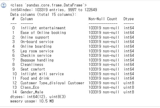
[복습] Logistic Regression 모델 결과
복습을 할 겸 Logistic Regression 를 진행해보자
from sklearn.linear_model import LogisticRegression
from sklearn.metrics import accuracy_score

# 선형 회귀 모델 초기화 및 학습
logistic_reg = LogisticRegression()
예측 수행
# 예측 수행
y_train_pred_logis = logistic_reg.predict(X_train)
y_test_pred_logis = logistic_reg.predict(X_test)

# 평가 지표 계산: 정확도 (맞은수/전체)
acc_train = accuracy_score(y_train, y_train_pred_logis)
acc_test = accuracy_score(y_test, y_test_pred_logis)

print(f'학습 데이터를 이용한 Acc 값 : {acc_train*100:.1f}%')
print(f'평가 데이터를 이용한 Acc 값 : {acc_test*100:.1f}%')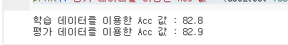
# Confusion matrix 생성을 위한 준비
from sklearn.metrics import confusion_matrix

cm_test_logis = confusion_matrix(y_test, y_test_pred_logis)

# 평가 데이터를 활용한 confusion matrix
import matplotlib.pyplot as plt

plt.imshow(cm_test_logis, interpolation='nearest', cmap='Blues')
plt.title("Logistic Reg. Confusion Matrix (Test)")
plt.colorbar()
tick_marks = np.arange(len(np.unique(y_test)))
plt.xticks(tick_marks, np.unique(y_test))
plt.yticks(tick_marks, np.unique(y_test))
plt.xlabel("Predicted Label")
plt.ylabel("True Label")

# 각 셀에 숫자 표시
for i in range(cm_test_logis.shape[0]):
    for j in range(cm_test_logis.shape[1]):
        plt.text(j, i, cm_test_logis[i, j], ha="center", va="center", color="black")

# 변수 영향력 시각화
plt.figure(figsize=(10, 6))
plt.barh(X_train.columns, logistic_reg.coef_.flatten())
plt.xlabel('Coefficient')
plt.ylabel('Features')
plt.title('Features Importance')
plt.show()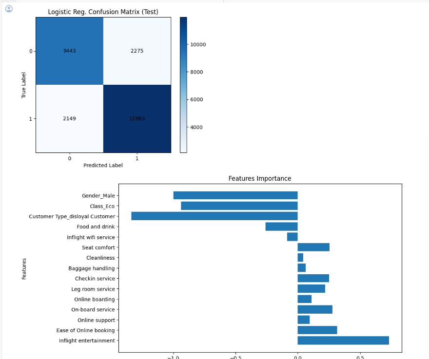
예측을 얼마나 잘했는지, 피쳐가 결과에 얼마나 영향을 끼치는지 를 볼 수 있다.
SVM 학습 진행
이제 SVM 학습을 진행해 보자
이론 시간에 좋은 성능을 보였던 RBF 커널을 활용해 학습
SVM 학습의 학습 시간은 선형 모델에 비해 오래 걸림
비행 만족도 데이터를 기준으로 약 30분 정도 소요
- %%timeit
• Jupyter Notebook에서 사용 가능
• 해당 셀을 실행하는데 걸린 시간 측정
• 셀 실행에 걸린 평균적인 시간과 sd 값을 표시
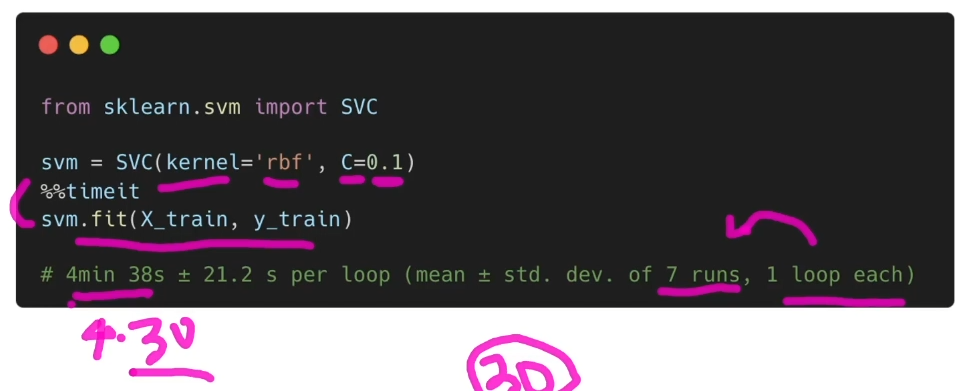
SVM 모델을 활용한 학습
from sklearn.svm import SVC

svm = SVC(kernel='rbf', C=0.1)
학습 SVM 모델을 활용한 예측 및 평가 진행
# 예측 수행
y_train_pred_svm = svm.predict(X_train)
y_test_pred_svm = svm.predict(X_test)

# 평가 지표 계산: 정확도 (맞은수/전체)
acc_train = accuracy_score(y_train, y_train_pred_svm)
acc_test = accuracy_score(y_test, y_test_pred_svm)

print(f'학습 데이터를 이용한 SVM Acc 값 : {acc_train*100:.1f}%')
print(f'평가 데이터를 이용한 SVM Acc 값 : {acc_test*100:.1f}%')
Logistic Regression 모델보다 10% 정도 느는 모습을 볼 수 있다!
새로운 분류 평가 척도 : 정밀도(Precision), 재현율 (Recall), F1 점수
SVM모델 평가 방법은 다양하다.
- 정밀도 (precision)
• 예측한 양성 결과가 실제로 얼마나 진짜 양성인지를 계산
• 모델이 양성 결과를 잘 찾아내야 하는 상황에서 중요
슛을 쏴서 얼마나 골을 넣었는지!
100% 감기 일때 알려주는! - 재현율 (recall)
• 실제 양성 중 얼마나 양성을 잘 찾아냈는지를 계산
• 정답을 잘 찾아내는 과정에서 중요
슛을 얼마나 많이 쐈는지!
암일 확률이 높을 때 알려주는! - F1 점수
• 정밀도와 재현율의 조화 평균
• 조화 평균을 사용해 낮음 점수에 대한 패널티를 늘림
• 정밀도와 재현율이 전반적으로 좋아야 좋은 F1값을 갖을 수 있음
정밀도, 재현율, F1 값 비교
# 정밀도, 재현율, F1 값 비교
from sklearn.metrics import precision_score, recall_score, f1_score

logistic_precision = precision_score(y_test, y_test_pred_logis)
logistic_recall = recall_score(y_test, y_test_pred_logis)
logistic_f1 = f1_score(y_test, y_test_pred_logis)
print(f'Logistic의 P,R,F1 : {logistic_precision:.2f} / {logistic_recall:.2f} / {logistic_f1:.2f}')

svm_precision = precision_score(y_test, y_test_pred_svm)
svm_recall = recall_score(y_test, y_test_pred_svm)
svm_f1 = f1_score(y_test, y_test_pred_svm)
print(f'SVM의 P,R,F1 : {svm_precision:.2f} / {svm_recall:.2f} / {svm_f1:.2f}')
WVM이 모두의 평가 방법에서 다 높게 나온다.
Decision Tree 모델을 활용한 학습
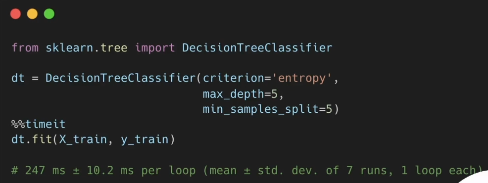
Entropy 결정 경계를 사용하는 최대 깊이 5의 Tree를 생성
- Decision Tree의 학습 시간은 SVM에 비해 짧음
- Tree를 구성하는 깊이에 따라 변동성이 크지만 일반적으로
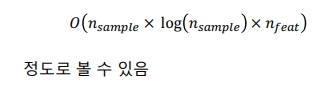
최고의 모델을 찾아서!
위에서 Decision Tree 모델의 depth를 5로 주었다.
왜일까!
머신러닝 모델의 크기가 커지고 복잡도가 증가하면 모델의 성능은 올라간다.
- 하지만 과적합(Overfitting) 현상이 발생하면 오히려 성능이 하락
• 학습 데이터에 대한 성능은 지속적으로 상승
• 평가 데이터에 대한 성능이 하락
• 학습 데이터를 단순히 암기하는 과정으로 돌입! - 따라서 평가 데이터에 대한 성능이 낮아지기 시작하는
지점의 세팅을 이용해 최적의 모델을 선택해야 함
• 옆 그림은 하이퍼파라메터 중 하나인
max depth 값을 이용한 서칭 그래프
# max depth에 따른 학습 결과 경향성 파악
max_depths = range(3, 30)

train_accuracies = []
test_accuracies = []

for depth in max_depths:
    model = DecisionTreeClassifier(criterion='entropy',
                                   max_depth=depth,
                                   min_samples_split=5)
    model.fit(X_train, y_train)

    # 학습 데이터에 대한 정확도
    y_train_pred = model.predict(X_train)
    train_acc = accuracy_score(y_train, y_train_pred)
    train_accuracies.append(train_acc)

    # 평가 데이터에 대한 정확도
    y_test_pred = model.predict(X_test)
    test_acc = accuracy_score(y_test, y_test_pred)
    test_accuracies.append(test_acc)

# 결과 시각화
plt.figure(figsize=(10, 6))
plt.plot(max_depths, train_accuracies, label='Training Accuracy')
plt.plot(max_depths, test_accuracies, label='Test Accuracy')
plt.xlabel('Max Depth')
plt.ylabel('Accuracy')
plt.title('Decision Tree Accuracy vs Max Depth')
plt.legend()
plt.show()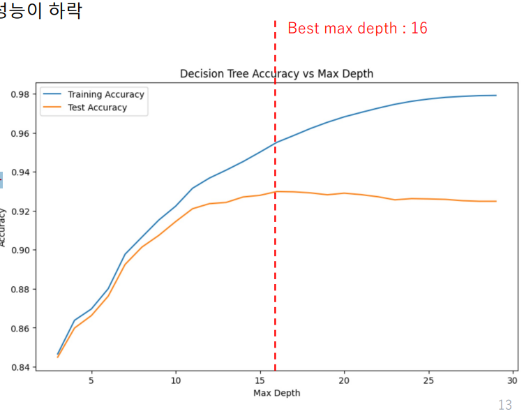
점선 이후 부분은 오버피팅 구간이라고 할 수 있다.
그렇기 때문에 death는 16이 가장 최적이라고 볼 수 있다.
숙제!
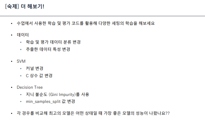
이건 나중에..

LV. 1