SVR (Support Vector Regresson)

회귀 문제에 적용되는 SVR

회귀 문제로 확장한 SVM 방법을 SVR (Support Vector Regression)이라고 함

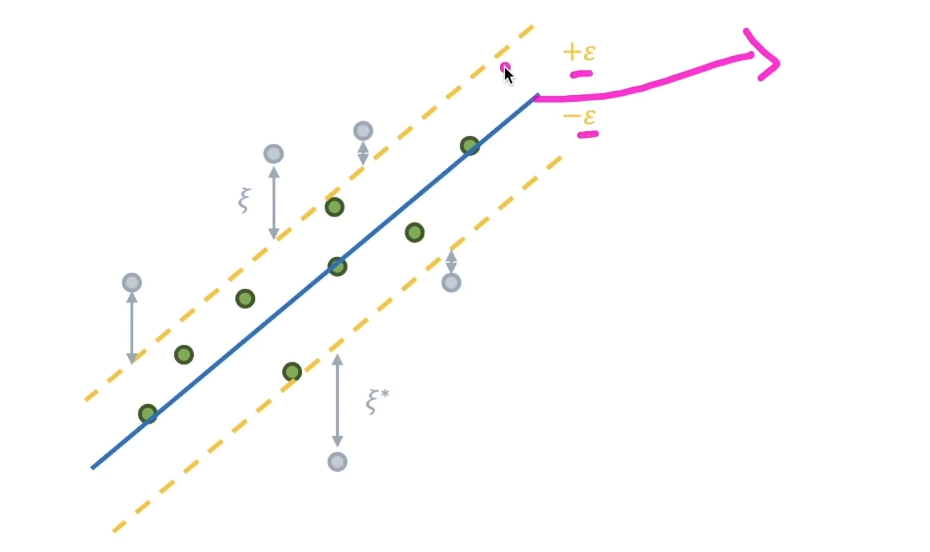
• 주어진 데이터에서 가능한 많은 데이터 포인트(초록색들)를 포함하는 마진 구역을 설정
  • 이 마진 구역은 사용자가 선언한 허용 오차내부의 구역
• 그 마진 구역 안에서 회귀선(혹은 초평면)을 찾는 것을 목표로 함

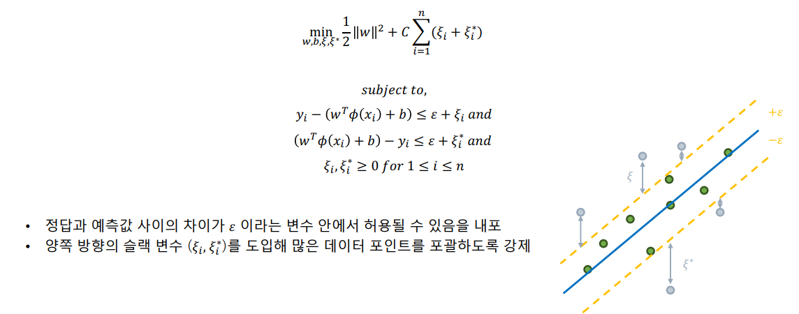
SVR의 최적화 문제

커널 함수를 적용한 SVR의 최적화 함수는 아래와 같음

SVR 실습

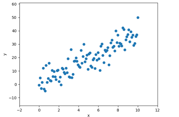
위와 같은 데이터를 가지고 SVR을 만들어 보자.

• SVR 함수를 호출!
• epsilon = : 어느 정도의 범위를 줄 것인지 선언.

from sklearn.svm import SVR

epsilon = 5

# SVR 객체 생성
svr_linear = SVR(kernel='linear', epsilon=epsilon)
svr_poly = SVR(kernel='poly', degree=3, epsilon=epsilon)
svr_rbf = SVR(kernel='rbf', epsilon=epsilon)
svr_sigmoid = SVR(kernel='sigmoid', epsilon=epsilon)

• SVR 모델 학습

# SVR 모델 학습
svr_linear.fit(x.reshape(-1, 1), y)
svr_poly.fit(x.reshape(-1, 1), y)
svr_rbf.fit(x.reshape(-1, 1), y)
svr_sigmoid.fit(x.reshape(-1, 1), y)

이후 시각화를 진행하면

# 그림을 그리기 위한 X 좌표 생성
x_range = np.linspace(x.min(), x.max(), 100).reshape(-1, 1)

# X 좌표에 대한 Y 출력 결과 도출
y_linear = svr_linear.predict(x_range)
y_poly = svr_poly.predict(x_range)
y_rbf = svr_rbf.predict(x_range)
y_sigmoid = svr_sigmoid.predict(x_range)

plt.figure(figsize=(12, 12))

# Linear 커널
plt.subplot(2, 2, 1)
plt.scatter(x, y)
plt.plot(x_range, y_linear, color='red')
plt.fill_between(x_range.ravel(), y_linear - svr_linear.epsilon, y_linear + svr_linear.epsilon, color='red', alpha=0.2)
plt.title("Linear SVR")
plt.xlabel('x')
plt.ylabel('y')

# Polynomial 커널
plt.subplot(2, 2, 2)
plt.scatter(x, y)
plt.plot(x_range, y_poly, color='red')
plt.fill_between(x_range.ravel(), y_poly - svr_poly.epsilon, y_poly + svr_poly.epsilon, color='red', alpha=0.2)
plt.title("Polynomial SVR")
plt.xlabel('x')
plt.ylabel('y')

# RBF 커널
plt.subplot(2, 2, 3)
plt.scatter(x, y)
plt.plot(x_range, y_rbf, color='red')
plt.fill_between(x_range.ravel(), y_rbf - svr_rbf.epsilon, y_rbf + svr_rbf.epsilon, color='red', alpha=0.2)
plt.title("RBF SVR")
plt.xlabel('x')
plt.ylabel('y')

# Sigmoid 커널
plt.subplot(2, 2, 4)
plt.scatter(x, y)
plt.plot(x_range, y_sigmoid, color='red')
plt.fill_between(x_range.ravel(), y_sigmoid - svr_sigmoid.epsilon, y_sigmoid + svr_sigmoid.epsilon, color='red', alpha=0.2)
plt.title("Sigmoid SVR")
plt.xlabel('x')
plt.ylabel('y')

plt.tight_layout()
plt.show()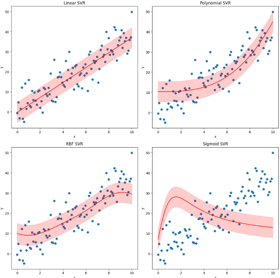

Linear과 RBF에서 데이터 포인트를 기준으로 선이 잘 만들어 진 것을 볼 수 있다.