SLAYER: Spike Layer Error Reassignment in Time(논문)

A new general backpropagation mechanism for learning synaptic weights and axonal delays which overcomes the problem of non-differentiability of the spike function and uses a temporal credit assignment policy for backpropagating error to preceding layers.

ANNs

• image classification and object recognition, to object tracking, signal processing, natural language processing, self driving cars, health care diagnostics, and many more.

backpropagation of error signal to the neurons in preceding layer

순전파(Forward Propagation)는 입력층에서 출력층으로 계산하며, 쉽게 예측값을 구하는 과정을 뜻합니다.

역전파(Back propagation)는 순전파와 반대로 출력증에서 입력층 방향으로 계산하며 가중치를 업데이트합니다.

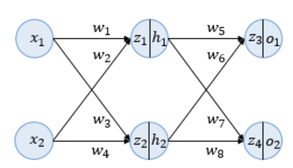
순전파

• 변수 z는 이전층의 입력값과 가중치를 모두 곱한 가중합을 의미합니다.
  z는 아직 활성화 함수인 sigmoid 함수를 거치지 않은 상태로, sigmoid 함수의 입력값을 의미합니다.

• z 우측에 존재하는 h와 o는 sigmoid 함수를 거친 값으로 각 뉴런의 출력값입니다.

Sigmoid function = $\frac{1}{1+e^{-x}}$

• h는 hidden layer, o는 out layer를 의미하며 편향 b는 고려하지 않습니다.

$o_1, o_2$는 예측값. 예측값과 실제값의 오차를 계산하기 위해서 Mean Square Error(MSE)를 사용.

MSE = $\frac{1}{N}\sum^N_{i=1}{(y^i-\hat{y})^2}$

$E_{o1}$ = $\frac{1}{2}(실제값_{o1}-예측값_{o1})^2$
$E_{o2}$ = $\frac{1}{2}(실제값_{o2}-예측값_{o2})^2$

$E_{total} = E_{o1} + E_{o2}$

역전파

chain rule을 이용해서, 새로운 가중치 값들을 갱신.

SNNs are similar to ANNs in terms of network topology, but differ in the choice of neuron model.

• (SNNs)Spiking neurons have memory and use a non-differentiable spiking neuron model (spike function)
• While ANNs typically have no memory and model each neuron using a continuously differentiable activation function.

Spike LAYer Error Reassignment (SLAYER).

SLAYER distributes the credit of error back through the SNN layers, much like the traditional backprop algorithm distributes error back through an ANN’s layers.

An SNN is a type of ANN that uses more biologically realistic spiking neurons, as its computational units.

Spiking Neuron Model

input spike, $S_i(t) = \sum_f{\delta(t-t_i^{(f)})}$

$t_i^{(f)}$ is the time of the $f^{(th)}$ spike of the $i^{th}$ input.

input spike converts into spike response signal by convolving $s_i(t)$ with a spike response kernel $\varepsilon$.

$a_i(t) = (ε ∗ s_i)(t)$

refractory response of neuron
(ν ∗ s)(t)
,where ν(·) is the refractory kernel and s(t) is the neuron’s output spike train.

Sum of Post Synaptic Potential (PSP), u(t) is

u(t) = $\sum{w_i} (ε ∗ s_i)(t) + (ν ∗ s)(t) = w^Ta(t) + (ν ∗ s)(t)$

can be extended with the axonal dealy,

as εd(t) = ε(t − d), where d ≥ 0 is the axonal delay

Backpropagation in SNN

Existing Methods

1) ANN to train an equivalent shadow network.

• training ANN and converting into SNN with some loss of accuracy.

(loss of accuracy)

• introducing extra constraints on neuron firing rate,scaling the weights, constraining the network parameters, formulating an equivalent transfer function for a spiking neuron, adding noise in the model, using probabilistic weights and so on.

2), and 3) directly on the SNN but differ in how they approximate the derivative of the spike function.

2) track of the membrane potential of spiking neurons only at spike times and backpropagates errors based only on membrane potentials at spike times.

ex) SpikeProp and its derivatives.
These methods are prone to the “dead neuron” problem:
when no neurons spike, no learning occurs. Heuristic measures are required to revive the network from such a condition.

3) the membrane potential of a spiking neuron at a single time step only.

Backpropagation using SLAYER

The Loss Function

how error is assigned to previous time points

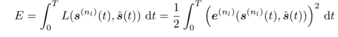
where $\hat{s}(t)$ is the target spike train, $L(S^(nl)(t), \hat{s}(t))$ is the loss at time instance t and $e^{(n1)}(S^{(n1)}(t), \hat{s}(t))$ is the error signal at the final layer.

A decision is typically made based on the number of output spikes during an interval rather than the precise timing of the spikes. why?

Experiments

Poisson distribution

Similarly a target spike train was generated using a Poisson distribution. The task is to learn to fire the desired spike train for the random spike inputs using an SNN with 25 hidden neurons.

MNIST Digit Classification

MNIST is a popular machine learning dataset.
Since SLAYER is a spike based learning algorithm, the images are converted into spike trains spanning 25 ms using Generalized Integrate and Fire Model of neuron

Use spike counting strategy.

NMNIST Digit Classification

This dataset is harder than MNIST because one has to deal with saccadic motion.

DVS Gesture Classification

Use DVS(Dynamic Vision Sensor), 사람의 홍채가 정보를 받아들이는 방식을 채택

• 기본 vision sensor은 모든 정보, 이미지를 저장함. 연속된 이미지를 영상화시키는 방식으로 카메라 작동. (저장공간, 시간, 동력 낭비)

• DVS는 기존의 영상화 된 프레임을 움직이는 사건이 발생할 때만 전송

Goal : Classifying the action sequence video into an action label.

data set (initialize)

29 images.(first 23 training, last 6 for testing)

True, 180 spikes
False, 30 spikes

TIDIGITS Classification

an audio classification dataset containing audio signals corresponding to digit utterances from ‘zero’ to ‘nine’ and ‘oh’.

The development of a CUDA accelerated learning framework for SLAYER was instrumental in tackling bigger datasets in SNN domain, although they are still not big when compared to the huge datasets tackled by conventional (non-spiking) deep learning.

TrueNorth, SpiNNaker, Intel Loihi와 같은 신경형 하드웨어는 극도로 저전력 칩에서 대규모 스파이킹 신경망을 구현할 수 있는 잠재력 을 보여줍니다. 이 칩들은 일반적으로 학습 메커니즘을 갖지 않거나 기본적인 학습 메커니즘을 내장하고 있습니다. 학습은 일반적으로 오프라인에서 이루어져야 합니다. SLAYER는 칩에 배포되기 전에 네트워크를 구성하기 위한 오프라인 훈련 시스템으로 활용할 수 있는 좋은 잠재력을 가지고 있습니다.

기본적인 학습 메커니즘의 내장 & 자기 학습
Intel Loihi(self-learning)