Stanford CS224W Machine Learning with Graphs Fall 2024/25
Why Graphs?
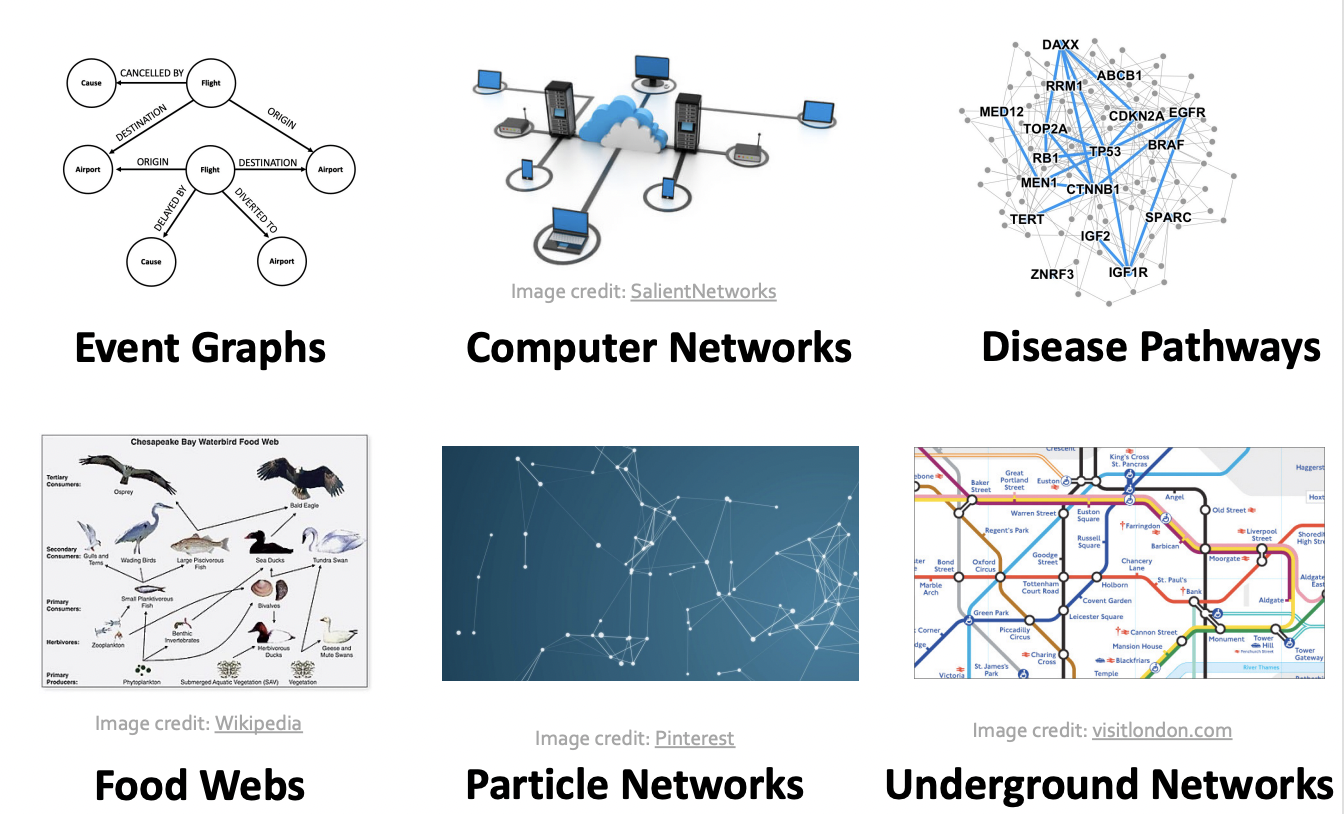
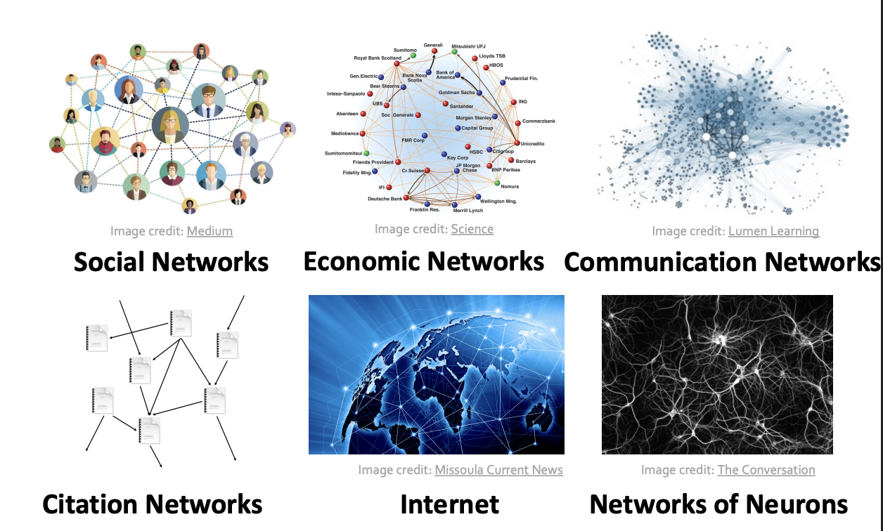
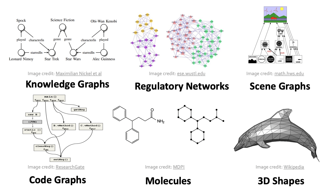
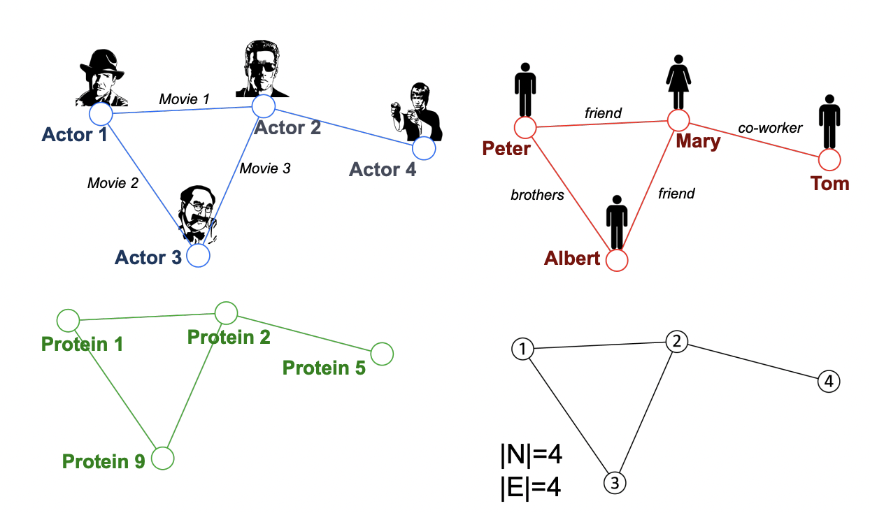
Graphs are a general language for describing and analyzing wntities with relations / interactions
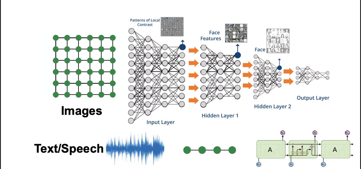
Many types of Data are graphs
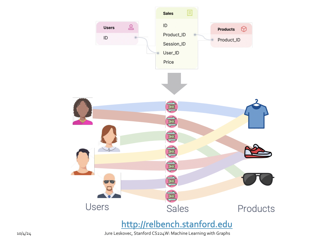
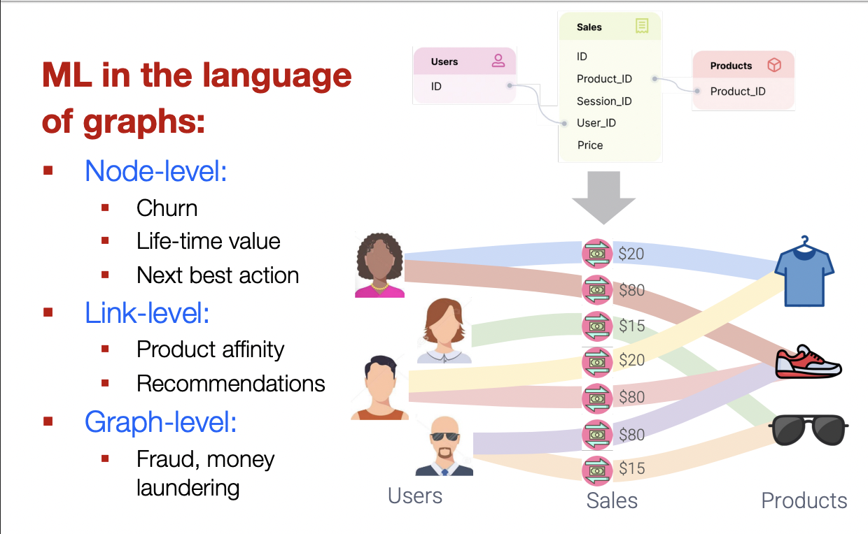
Database are Graphs
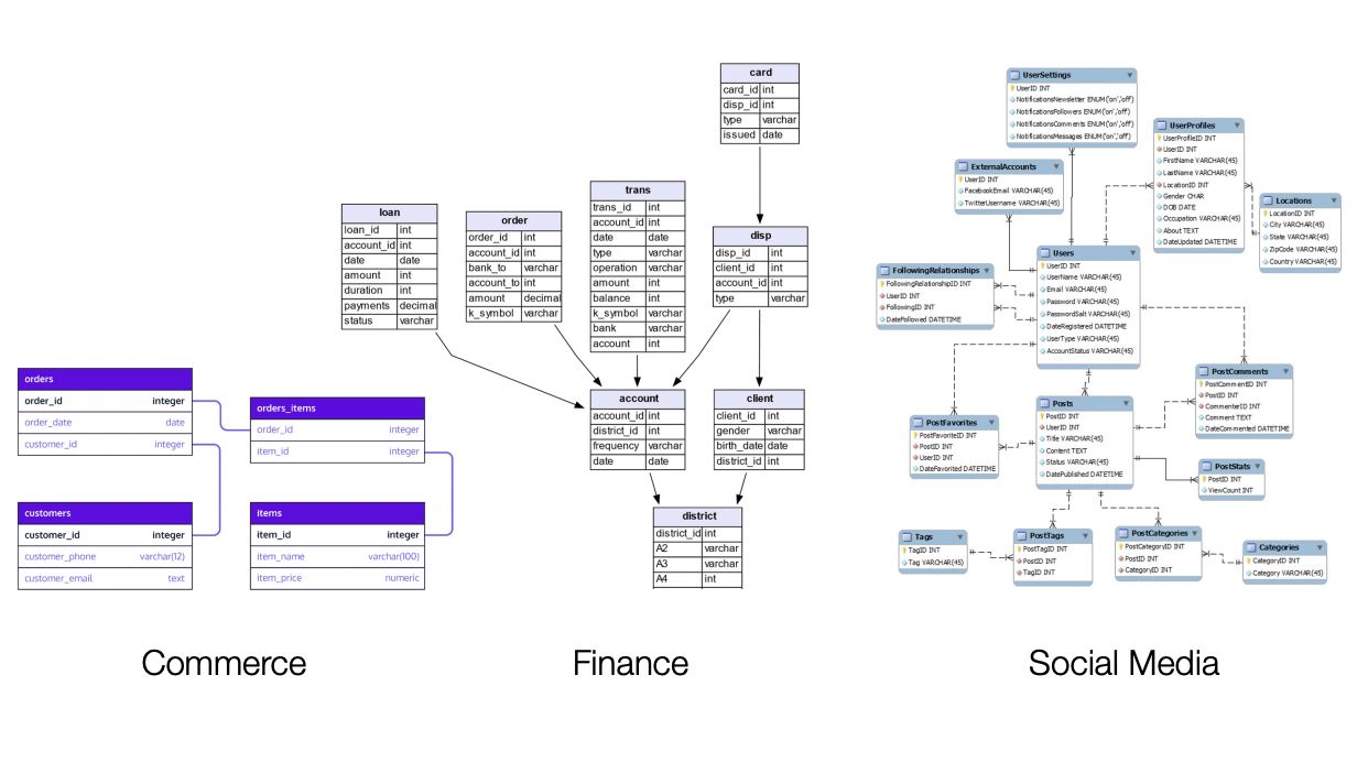
Relational Deep Learning
Graphs : Machine Learning
복잡한 영역은 풍부한 관계구조를 가지고 있으며, 이는 relational graph 형태로 표현될 수 있습니다.
관계를 명시적으로 모델링함으로써, 더 나은 성능을 얻을 수 있습니다.
main question :
우리는 더 나은 예측을 위해 이러한 관계 구조를 어떻게 활용할 수 있을까?
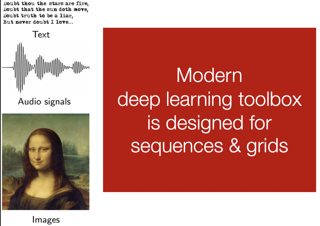
Modern ML toolbox
Why is Graph Deep Learning Hard?
Networks are complex
- Arbitraty size and complex topological structure.
(i.e., no spatial localuty like grids)
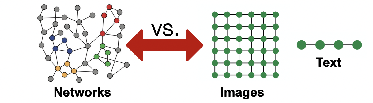
- No fixed node ordering or reference point
- Often dynamic and have multinodal features
How can we develop neural networks that are much more broadly applicable?
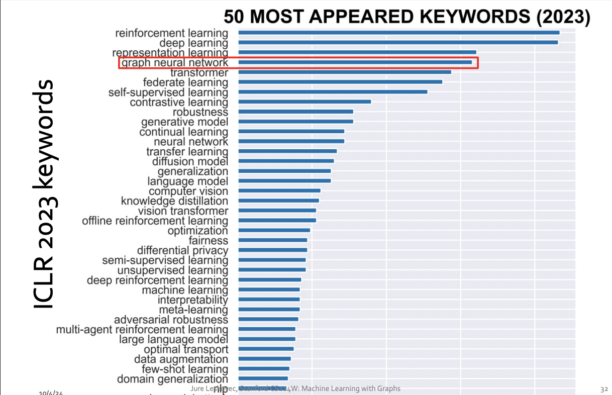
Graphs are the new frontier of deep learning
How subfield in ML
Choice of Graph Representation
Graphs : A common Language
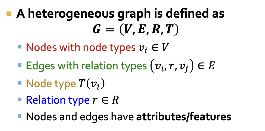
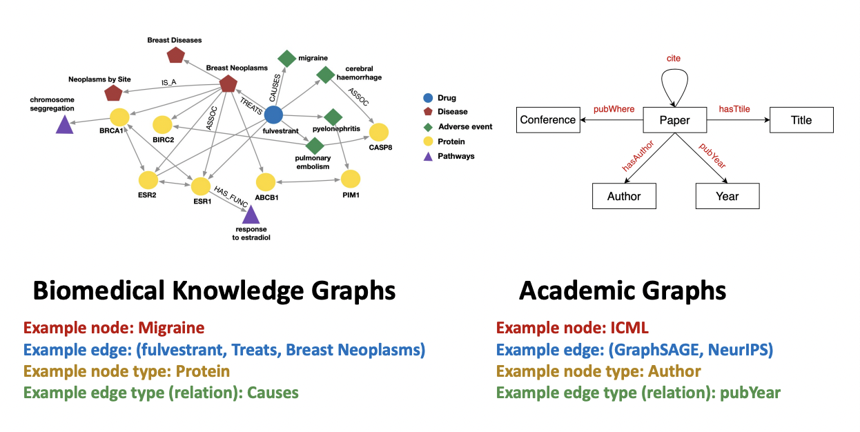
Heterogeneous Graphs
적절한 그래프 표현(Representation) 선택하기
- 그래프를 어떻게 구축할 것인가?
- 노드는 무엇인가- 엣지는 무엇인가
- 특정 도메인/문제에 대해 올바른 네트워크 표현을 선택하는 것은, 그 네트워크를 성공적으로 활용할 수 있는 능력을 결정한다
- 어떤 경우에는 하나의 명확하고 유일한 표현이 존재한다.
- 다른 경우에는 표현이 여러 가지로 가능하며, 유일하지 않다.
- 링크(엣지)를 어떻게 설정하느냐에 따라, 연구할 수 있는 문제의 성격이 결정된다
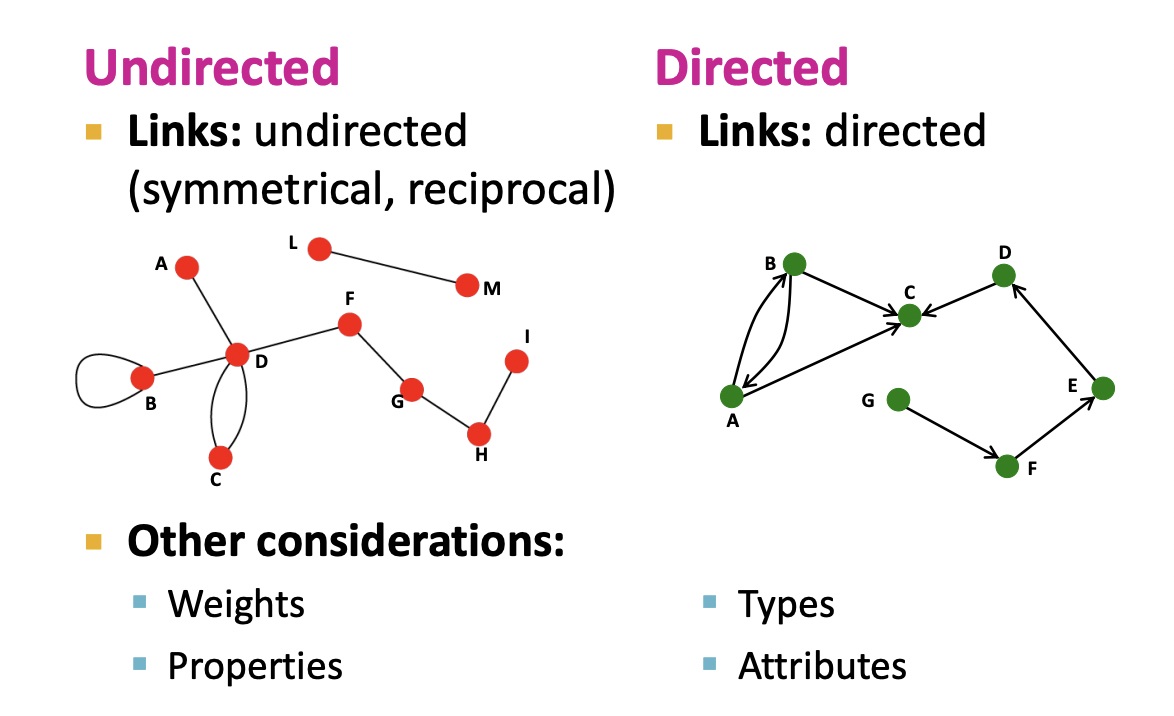
Directed vs. Undirected Graphs
Bipartite Graph
Applications of Graph ML
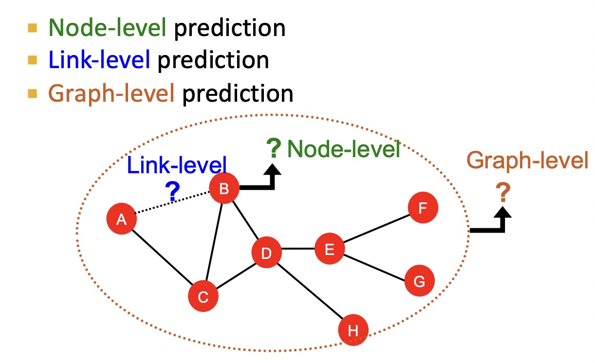
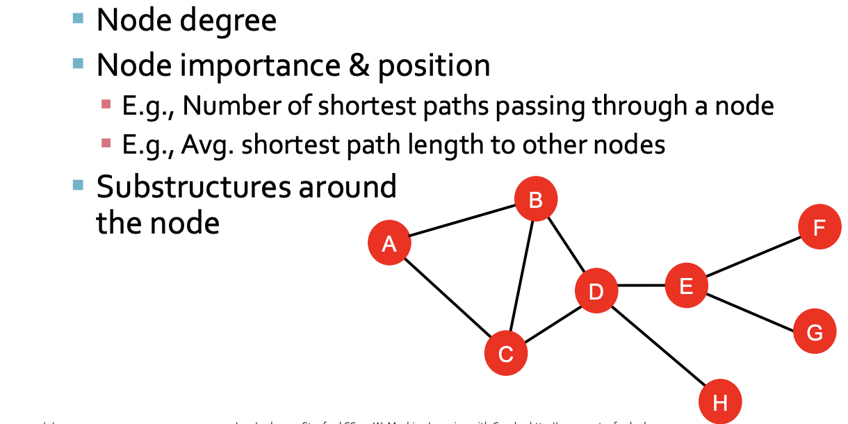
Node-Level Tasks
Node-Level Network Structure
Goal : Characterize the structure and position of a node in the network
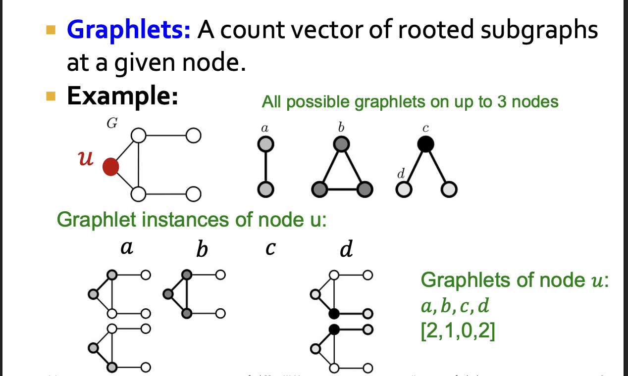
Node's Subgraphs : Graphlets
Discussion
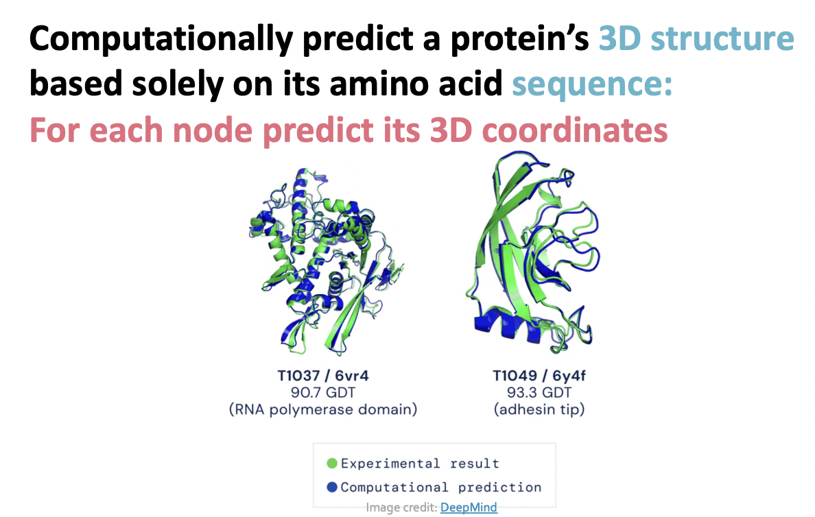
Protein Folding
AlphaFold : Impact
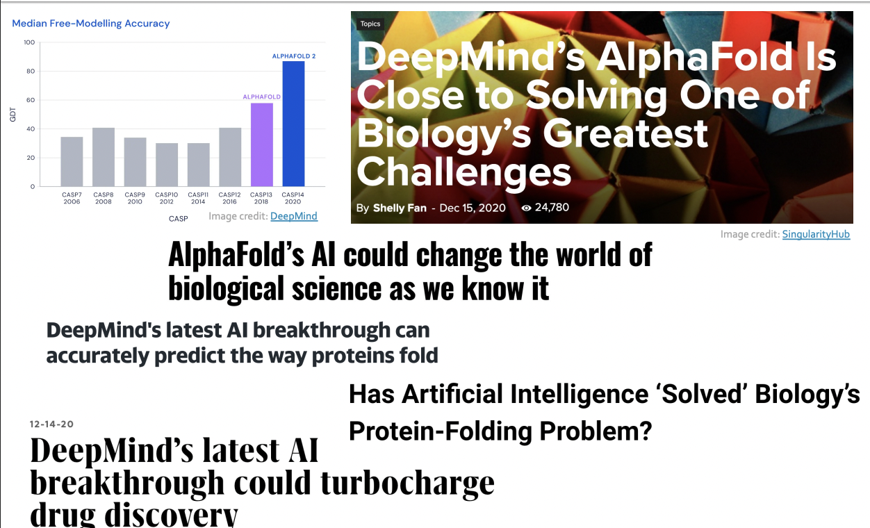
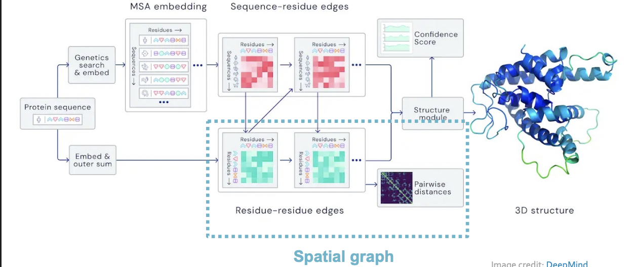
AlphaFold : Solving Protein Folding
- Key idea : "Spatial Graph"
- Nodes : Amino acids in a protein sequence
- Edges : Proximity between amino acids (residues)
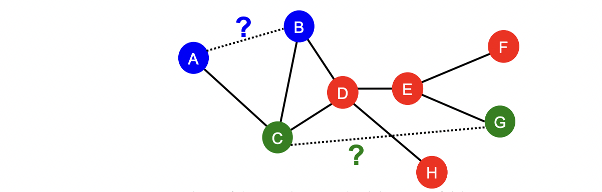
Link Prediction
Link-Level Prediction Task
- The task is to predict new/missing/unknown links based on the existing links.
- At test time, node pairs (with no existing links) are ranked, and top K node pairs ar predicted
- Task : Make a prediction for a pair of nodes
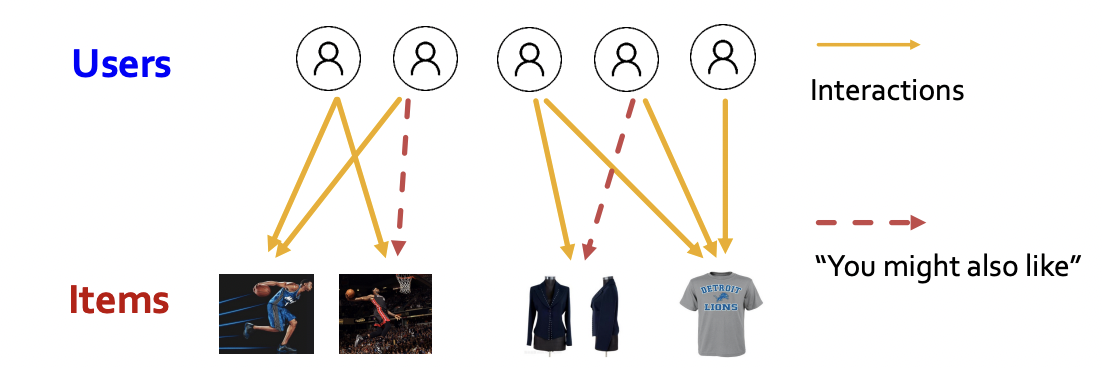
Recommender Systems
- Users interacts with items
- watch movies, buy merchandise, listen to music
- Nodes : Users and items
- Edges : User-item interactions
- Goal : Recommend items users might like
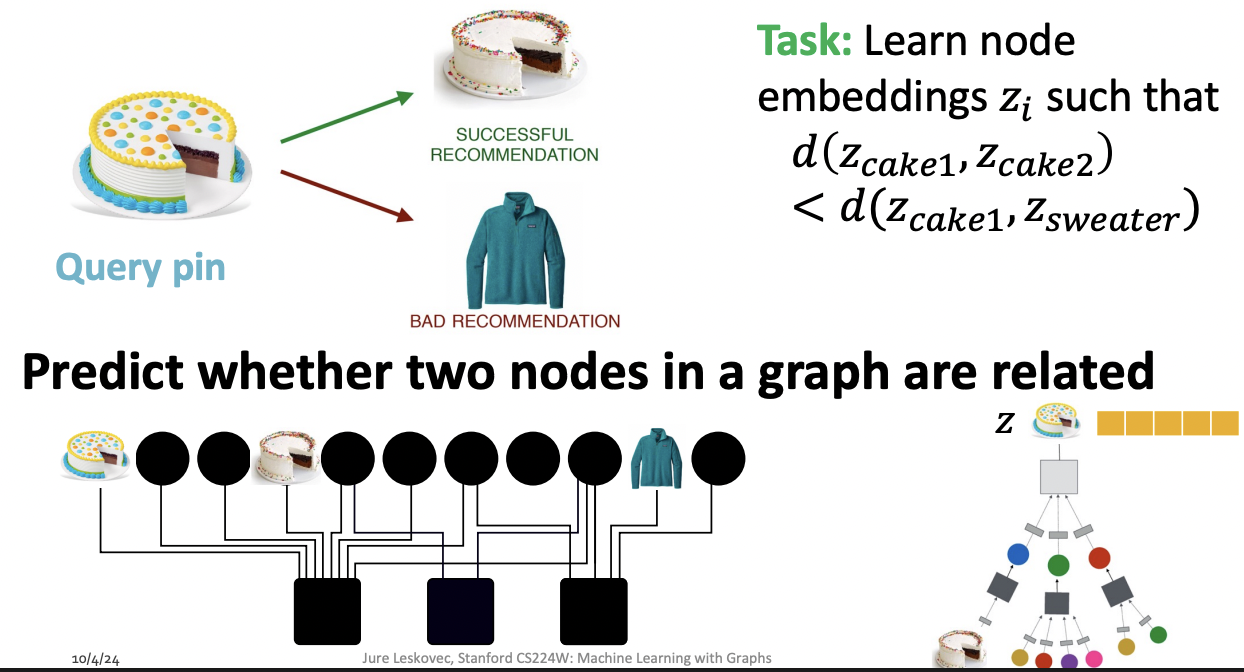
PinSage : Graph-based Recommender
- Task : Recommend related pins to users
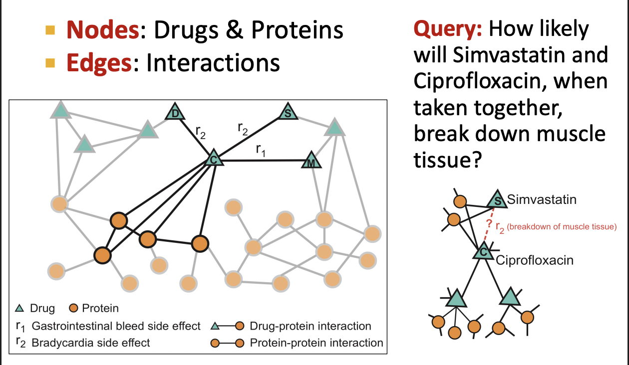
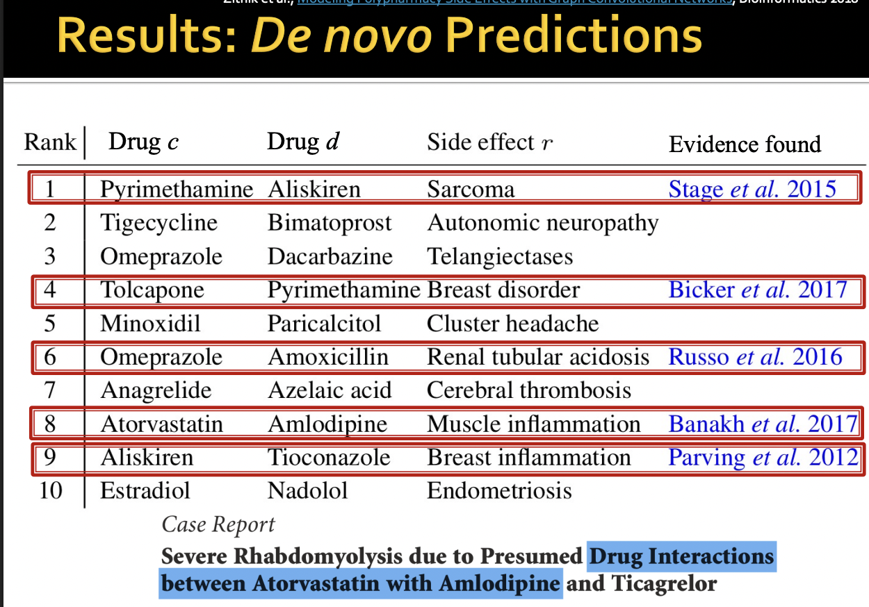
Drug Side Effects
Many patients take multiple drugs to treat complex or co-existing diseases:
- 46% of people ages 70-79 take more than 5 drugs
- Many patients take more than 20 drugs to treat heart disease, depression, insomnia, etc.
Task : Given a pair of drugs predict adverse side effects
Biomedical Graph Link Prediction
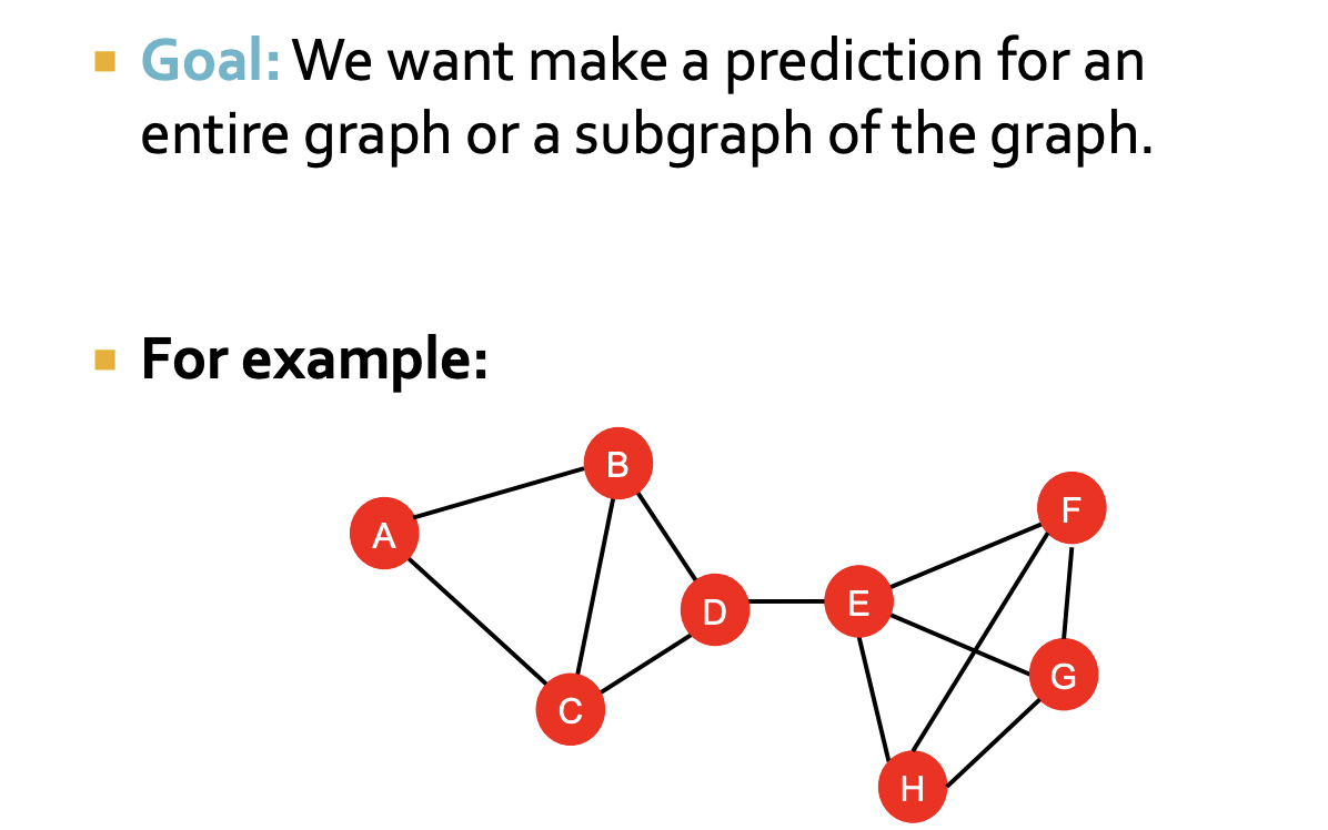
Graph-Level Tasks
Graph - Level Prediction
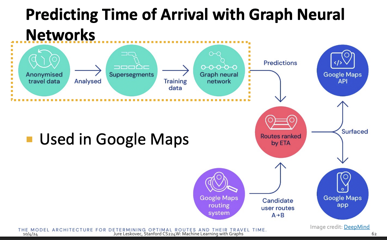
Traffic Prediction
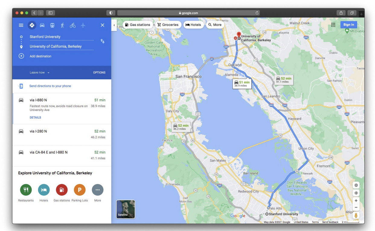
Road Network as a Graph
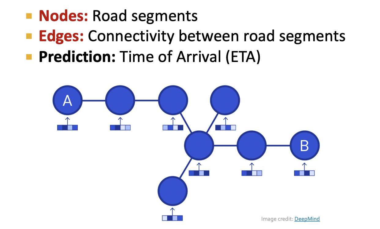
Traffic Prediction via GNN
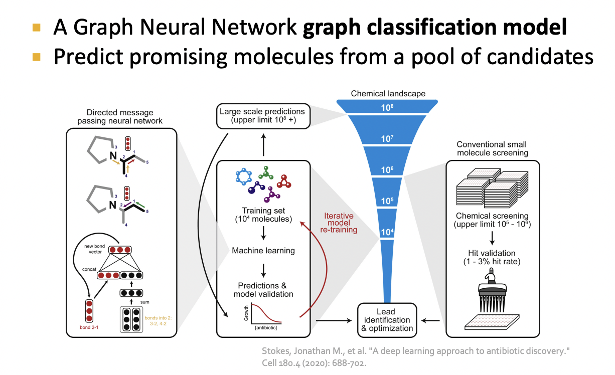
Drug Discovery
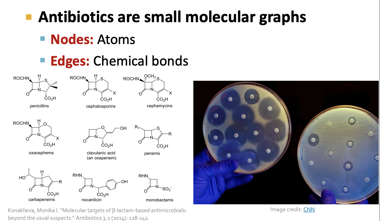
Deep Learning for Antibiotic Discovery
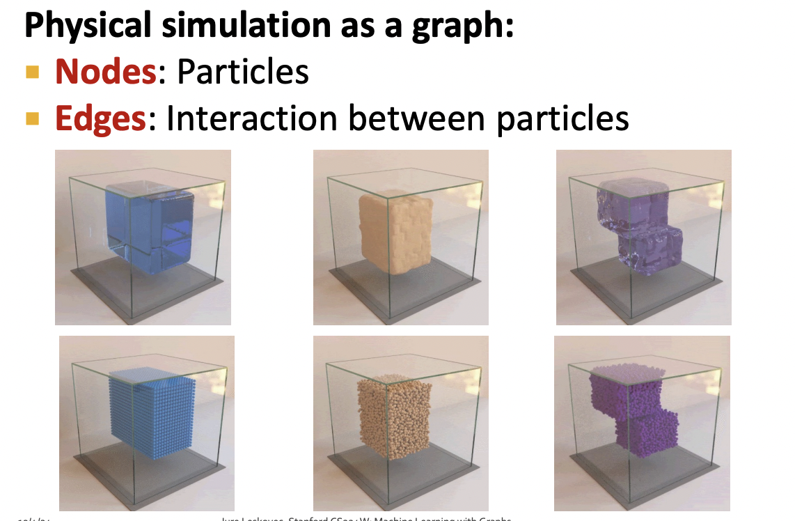
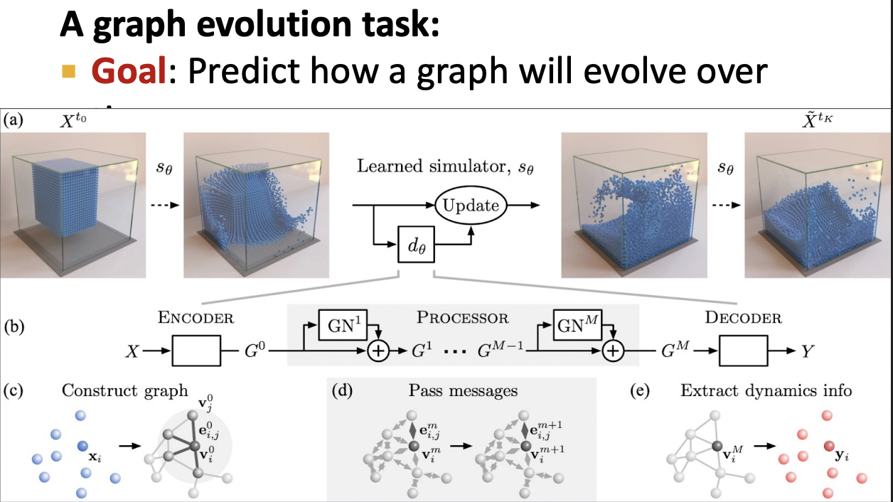
Physics Simulation
Simulation Learning Framework
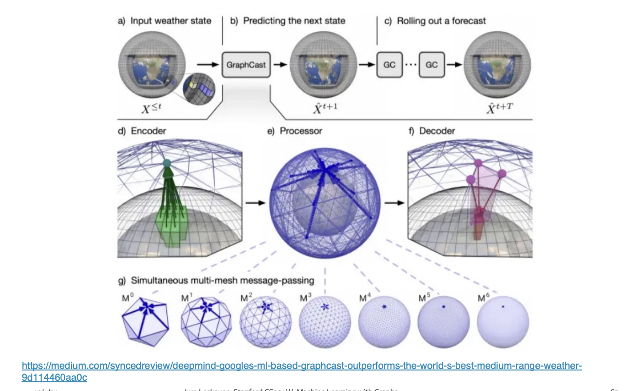
Application : Weather forecasting
실습
Data 객체
PyG의 data 객체란?
- PyG에서 그래프 한 개를 표현하는 기본 단위
- 그래프 (노드 + 엣지 + 피처 + 라벨)을 한 덩어리로 묶은 컨테이너임.
- 하나의 그래프를 구성하고 있는 모든 정보 담은 객체
Data(edge_index=[2, 156], x=[34, 34], y=[34], train_mask=[34])
- edge_index : 연결 정보로 156개의 간선, 각 간선은 (출발노드, 도착노드) 쌍으로 표현 2x156 행렬
- x : 노드 피처 -> 각 노드의 특징 벡터 (34개 노드, 각 노트마다 34 차원 feature vector)
- y : 노드 라벨 -> 각 노드 클래스 레이블
- train_mask : 학습 데이터 마스크 -> 어떤 노드를 학습에 사용할 지 표시하는 Boolean 벡터
Edge Index
from IPython.display import Javascript  # Restrict height of output cell.
display(Javascript('''google.colab.output.setIframeHeight(0, true, {maxHeight: 300})'''))

edge_index = data.edge_index
print(edge_index.t())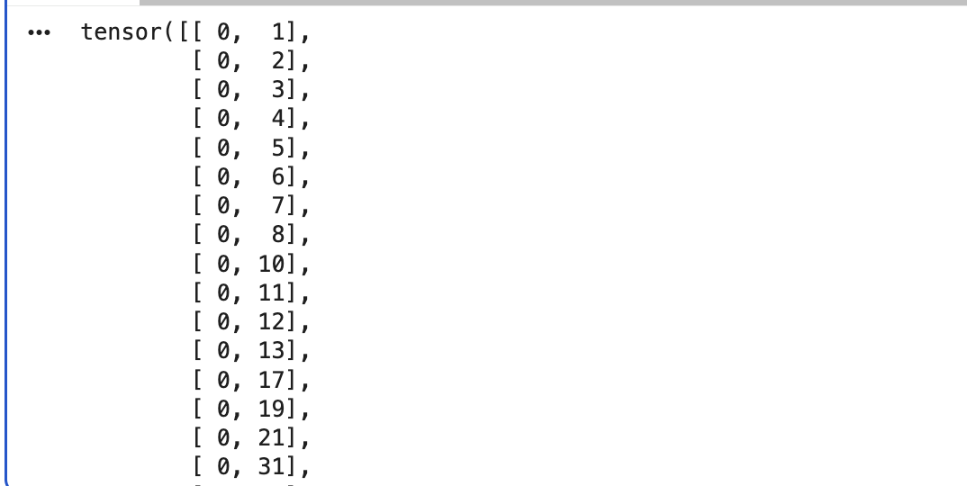
- 그래프 데이터는 edge_index 형태로 출력해야 하는건가??
edge_index를 출력해보면, PyTorch Geometric이 그래프의 연결 관계를 내부적으로 어떻게 표현하는지 더 잘 이해가능함. - 각 edge는 두 개의 노드 인덱스로 이뤄진 튜플로 표현됨.
edge_index의 첫 번째 값은 source node의 인덱스 표현
edge_index의 두 번째 값은 destination node의 인덱스 표현 - 이러한 표현 방식은 sparse matrix 표현 시 자주 사용되는 COO(Coordinate) 형식으로 알려짐
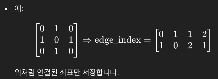
COO 포맷?
- 전체 adjacency matrix 저장하지 않고, 연결된 노드 쌍만 (row, column) 형태로 저장하는 방식
- 메모리 사용량이 훨씬 줄어든다.
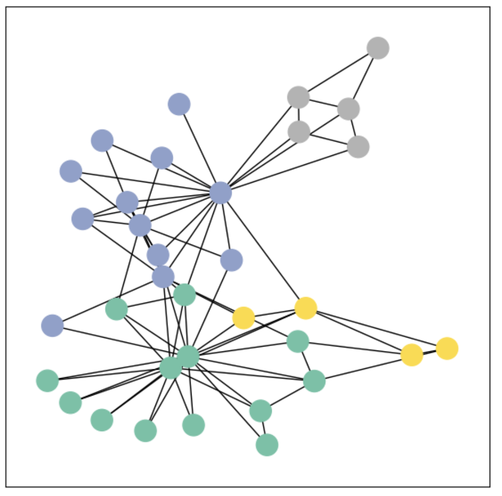
시각화
PyG의 그래프를 networkx 형식으로 변환하면 그래프 조작뿐만 아니라 시각화를 위한 강력한 기능들을 사용할 수 있음.
from torch_geometric.utils import to_networkx

G = to_networkx(data, to_undirected=True)
visualize(G, color = data.y)
시각화 결과
Graph Neural Network (GNN) 구현하기
GCN 레이어 사용하기
GNN의 가장 기본적인 연산자 중 하나는 GCN (Graph Convolutional Network) 레이어.
GCNConv는 입력으로
- 노드 피처 행렬 x
- 그래프 연결 정보 edge_index (COO 포맷)을 받아 연산 수행
즉,
GNN의 출력은 무엇일까?
GNN의 목표는 입력 그래프
를 받아서,
각 노드 ( v_i \in V ) 에 대한 유용한 임베딩 벡터(embedding) 를 학습하는 것
각 노드는 초기 입력 피처
를 가지고 있으며,
우리가 학습하려는 함수는 다음과 같습니다:
즉,
노드와 그 피처 벡터(그리고 그래프 구조) 를 입력받아
해당 노드를 잘 표현할 수 있는 임베딩 벡터를 출력하는 함수임.
임베딩의 의미
이렇게 학습된 노드 임베딩은 그래프 내의 구조적, 의미적 정보를 반영한 벡터 표현으로, 다양한 downstream task에 활용 가능함.
예를 들어,
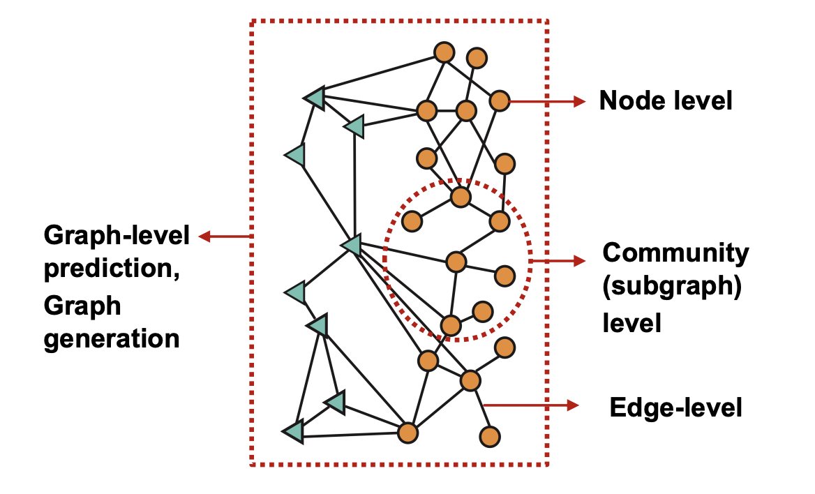
- 노드 수준 (Node-level) -> 커뮤니티 분류, 역할 예측
- 엣지 수준 (Edge-level) -> 링크 예측
- 그래프 수준 (Graph-level) -> 분자 특성 예측, 문서 분류 등
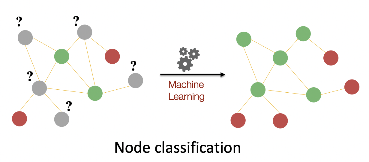
- 노드 분류 (Node Classification) 문제 다루기
- 즉, 그래프 내 각 노드를 어떤 커뮤니티에 속하는지 분류하는 것
import torch
from torch.nn import Linear # 선형 레이어 클래스
from torch_geometric.nn import GCNConv
# PyTorch Geometric에서 제공하는 그래프 합성곱(Graph Convolution) 레이어.
# 이 레이어는 인접행렬 정보를 이용해 이웃 노드의 특징을 집계하는 역할.

# 3층 GCN(Graph Convolutional Network) + 선형 분류기(classifier)
class GCN(torch.nn.Module): # GCN 신경망 클래스 정의 + torch.nn.Module을 상속받아서 PyTorch 모델처럼 작동하게 함.

    def __init__(self):
        super().__init__() # 부모 클래스 초기화(필수)
        torch.manual_seed(1234) # 랜덤 시드 고정하기 -> 동일한 초기 가중치 얻도록함
        self.conv1 = GCNConv(dataset.num_features, 4) # 노드 피처의 개수, 출력차원 = 4 -> 각 노드의 feature를 4차원 공간으로 투영
        self.conv2 = GCNConv(4, 4) # 2-hop 이웃 학습하기
        self.conv3 = GCNConv(4, 2) # 입력 4 -> 출력 2로 줄여서 최종 임베딩 공간으로 만듬.
        self.classifier = Linear(2, dataset.num_classes) # 마지막 선형 분류기 -> 입력 : 2차원 GNN 임베딩 , 출력 : 데이터셋의 클래스 개수 num_classes (각 노드를 어떤 클래스에 속하는 지 예측하기)

    def forward(self, x, edge_index): # 모델의 순전파를 정의하는 부분
        h = self.conv1(x, edge_index) # x: 각 노드의 feature matrix (shape: [num_nodes, num_features]), edge_index : 그래프의 연결구조 (shape: [2, num_edges], COO 형식)
        h = h.tanh() # 비선형 활성화 함수로, 값을 [-1,1] 범위로 제한
        h = self.conv2(h, edge_index)
        h = h.tanh()
        h = self.conv3(h, edge_index)
        h = h.tanh()  # Final GNN embedding space.

        # Apply a final (linear) classifier.
        out = self.classifier(h) # GCN에서 얻은 각 노드의 임베딩을 분류기에 통과시켜 클래스별 점수 (logit)을 출력함. out의 shape : [num_nodes, num_classes]

        return out, h
# 분류 결과와 마지막 임베딩을 반환
model = GCN()
print(model)- init 안에서 모든 구성 블록을 초기화하고 forward 함수에서 네트워크의 연산 흐름을 정의함.
- 그래프 합성곱 레이어 3개를 정의하고 쌓기 , 각 레이어는 각 노드 1-hop 이웃으로부터 정보를 집계함.
- 이 레이어들을 순차적으로 결합하면 각 노드가 최대 3-hop 이웃의 정보를 통합할 수 있게됨.
- 각 GCNConv 레이어는 노드 피처의 차원을 점점 줄이도록 설계되어 있음.
feature dimension : 34 -> 4 -> 4 -> 2 - 각 GCNConv 레이어 뒤에는 비선형 함수 tanh가 적용 -> 모델의 표현력을 높임
- torch.nn.Linear : 단일 선형 변환을 적용함.이 분류기는 각 노드를 4개의 클래스 중 하나로 매핑
- 최종 분류기의 출력과 GNN이 생성한 노드 임베딩 두 가지를 모두 반환함.
GNN의 귀납적 편향
model = GCN()

_, h = model(data.x, data.edge_index)
print(f'Embedding shape: {list(h.shape)}')

visualize(h, color=data.y)
Embedding shape: [34, 2]
- 모델의 가중치를 학습시키기도 전에, 모델이 생성한 노드 임베딩은 이미 그래프의 커뮤니티 구조를 잘 반영
- 같은 색에 속한 노드들이 임베딩 공간에서도 이미 가깝게 모여 있음.
- 이때 모델의 가중치는 완전히 무작위로 초기화된 상태이며, 아직 단 한 번의 학습도 진행하지 않은 상황
- 이 현상은 GNN이 매우 강력한 귀납적 편향을 가지고 있음을 의미함.
- 즉, 입력 그래프에서 서로 가까운 노드들은 모델이 학습하지 않아도 유사한 임베딩 표현을 가지도록 자연스럽게 설계되어 있다는 것을 의미함.
Karate Club Network에서의 학습
하지만 여기서 의문이 생길 수 있는데,
'과연 학습을 하면 더 좋아질까?'
- 그래프 내 4개의 노드에 대해 커뮤니티 레이블 (정답) 을 알고 있다고 가정하고, 이를 이용해 network parameter 학습시켜 보자
- 우리의 모델은 완전히 미분가능 + 파라미터화 -> 일부 노드에 레이블을 추가한 뒤 모델 학습 -> 노드 임베딩이 어떻게 변화하는 지 관찰 가능함.
- semi-supervised learning or transductive learning 사용
- 클래스당 단 1개의 노드만 이용해 학습을 수행하지만,- 그래프 전체의 구조 정보는 학습 과정에서 자유롭게 활용가능함.
GNN 학습 과정
모델 학습 과정은 일반적인 PyTorch 모델 학습과 거의 동일함.
- 네트워크 구조를 정의
- loss function 설정 (CrossEntropy loss)
- Stochastic Gradient Descent Optimizer 초기화
- 여러번의 최적화 반복
각 단계는
- forward pass (순전파) : 모델 예측 및 손실 계산
- backward pass (역전파) : 손실에 대한 가중치의 기울기 계산
Semi-supervised에서의 손실 계산
- semi-supervised 설정은 다음 코드 한 줄로 구현된다.
loss = criterion(out[data.train_mask], data.y[data.train_mask])- 여기서의 핵심은, 모델이 모든 노드의 임베딩을 계산하더라도 손실은 오직 훈련용 노드만 사용한다는 것
- out[data.train_mask] : 모델의 예측 결과 중 학습에 사용할 노드만 선택
- data.y[data.train_mask] : 해당 노드들의 정답 레이블만 선택
import time
from IPython.display import Javascript  # Restrict height of output cell.
display(Javascript('''google.colab.output.setIframeHeight(0, true, {maxHeight: 430})'''))

model = GCN()
criterion = torch.nn.CrossEntropyLoss()  # Define loss criterion.
optimizer = torch.optim.Adam(model.parameters(), lr=0.01)  # Define optimizer.

def train(data): # PyG의 Data 객체
    optimizer.zero_grad()  # Clear gradients.
    out, h = model(data.x, data.edge_index)  # Perform a single forward pass.
    loss = criterion(out[data.train_mask], data.y[data.train_mask])  # Compute the loss solely based on the training nodes.
    loss.backward()  # Derive gradients.
    optimizer.step()  # Update parameters based on gradients.

    accuracy = {}
    # Calculate training accuracy on our four examples
    predicted_classes = torch.argmax(out[data.train_mask], axis=1) # [0.6, 0.2, 0.7, 0.1] -> 2
    target_classes = data.y[data.train_mask]
    accuracy['train'] = torch.mean(
        torch.where(predicted_classes == target_classes, 1, 0).float())

    # Calculate validation accuracy on the whole graph
    predicted_classes = torch.argmax(out, axis=1)
    target_classes = data.y
    accuracy['val'] = torch.mean(
        torch.where(predicted_classes == target_classes, 1, 0).float())

    return loss, h, accuracy

for epoch in range(500): # 500번 반복 학습 (epoch = 전체 그래프 1회 학습 단위)
    loss, h, accuracy = train(data) # 매 epoch마다 train을 호출해서 손실 및 정확도 갱신
    # Visualize the node embeddings every 10 epochs
    if epoch % 10 == 0: # 10 epoch마다 한 번씩 노드 임베딩 시각화
        visualize(h, color=data.y, epoch=epoch, loss=loss, accuracy=accuracy) # 각 노드를 2D 좌표로 그려서, 같은 레이블 data.y끼리 색을 다르게 표현
        time.sleep(0.3) # 시각화 사이에 0.3초 대기 -> 애니메이션처럼 변화 과정을 볼 수 있게함
해석
- data.x : 노드 피처 행렬
- data.edge_index : 그래프 연결 정보
- data.y : 노드의 정답 레이블
- data.train_mask : 학습에 사용할 노드 인덱스
(1) 경사 초기화 및 Forward Pass
optimizer.zero_grad()
out, h = model(data.x, data.edge_index)
- optimizer.zero_grad() : 이전 단계에서 계산된 gradient(기울기)를 초기화 (PyTorch 학습의 기본)
- out, h = model(...) :
out: GCN의 최종 출력 (각 노드별 class 예측값 — logit)
h: 중간 임베딩 (2차원 feature representation)
(2) 손실 계산 (학습용 노드만 사용)
loss = criterion(out[data.train_mask], data.y[data.train_mask])
- train_mask = True인 노드만 선택해서 손실 계산
- 즉, 그래프 전체를 사용하지만, 오직 일부 노드의 정답만으로 학습하는 semi-parametric supervised learning
(3) Backward Pass (기울기 계산 및 업데이트)
loss.backward() # Derive gradients.
optimizer.step() # Update parameters based on gradients.
- loss.backward() : 손실값으로부터 모델 파라미터에 대한 기울기를 계산
- optimizer.step() : 기울기를 이용해 파라미터 업데이트 (Adam 방식)
(4) 정확도 계산 (Train & Validation)
accuracy = {}
- 딕셔너리로 학습 정확도와 검증 정확도를 따로 저장한다.
✅ 학습 데이터 정확도
predicted_classes = torch.argmax(out[data.train_mask], axis=1)
target_classes = data.y[data.train_mask]
accuracy['train'] = torch.mean(
torch.where(predicted_classes == target_classes, 1, 0).float())
- torch.argmax : 모델 출력 중 가장 높은 확률(class index)을 예측값으로 선택
- torch.where(predicted_classes == target_classes, 1, 0) : 맞춘 경우 1, 틀린 경우 0
- torch.mean(...) : 평균 → 전체 학습 노드 중 정확히 맞춘 비율
✅ 전체 그래프(Validation) 정확도
predicted_classes = torch.argmax(out, axis=1)
target_classes = data.y
accuracy['val'] = torch.mean(
torch.where(predicted_classes == target_classes, 1, 0).float())
- 이번엔 그래프의 모든 노드를 대상으로 예측값과 실제 레이블 비교
- 그래프 전체 수준에서의 정확도 계산 (validation 개념과 유사)
결과
-
As one can see, our 3-layer GCN model manages to separate the communities pretty well and classify most of the nodes correctly.
-
Furthermore, we did this all with a few lines of code, thanks to the PyTorch Geometric library which helped us out with data handling and GNN implementations.