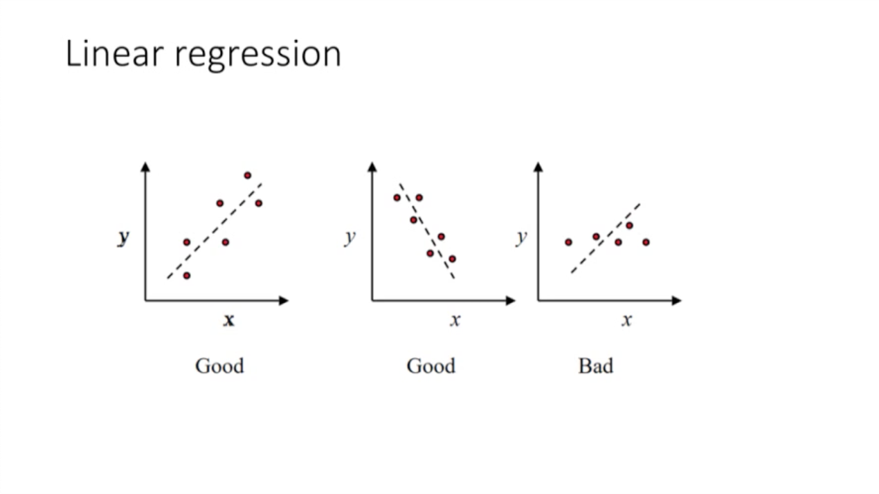
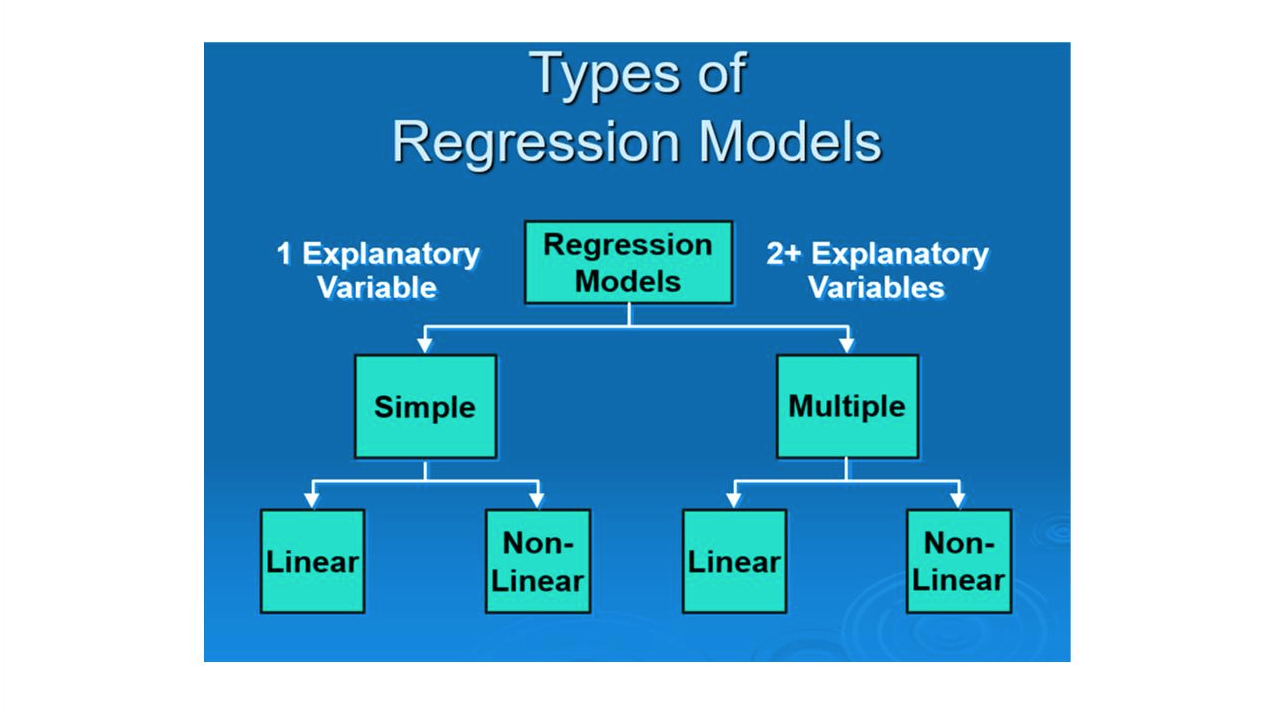
Linear regression
여러 데이터를 분석해서 오차가 가장 적은 하나의 직선을 구하는 것.
빅데이터, 인공지능에서 중요한 수치로 사용
개념 설명
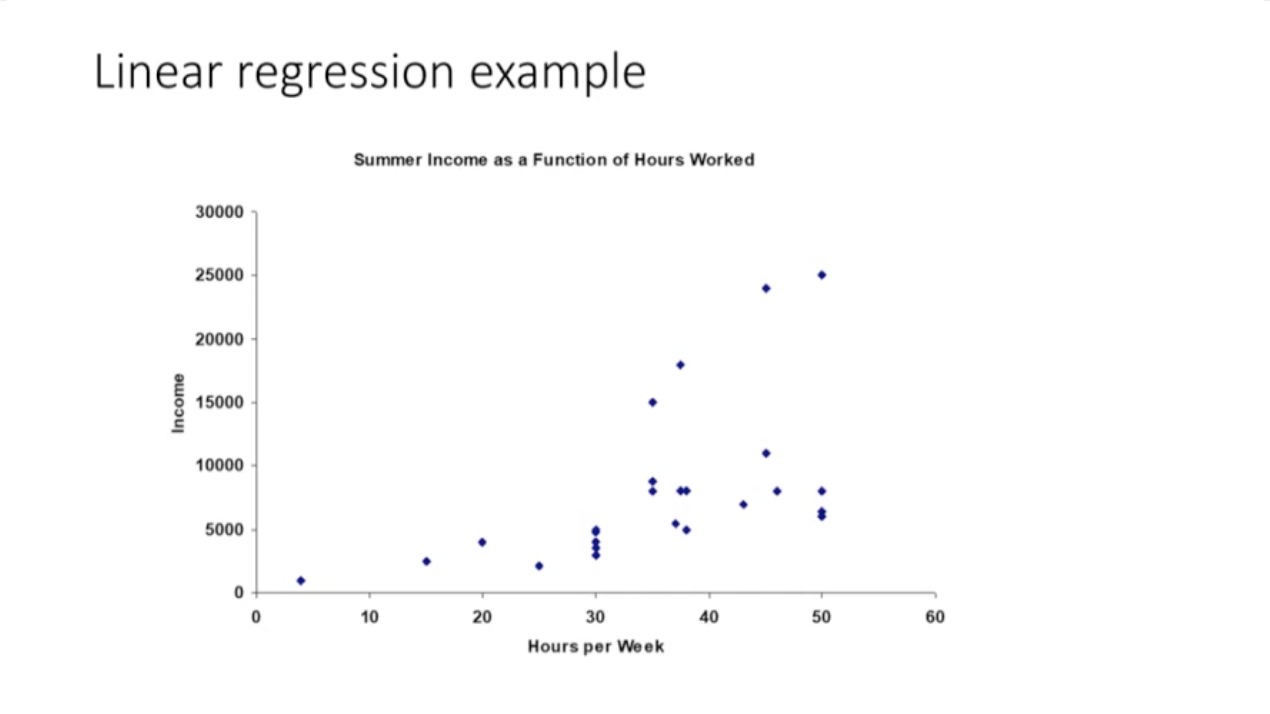
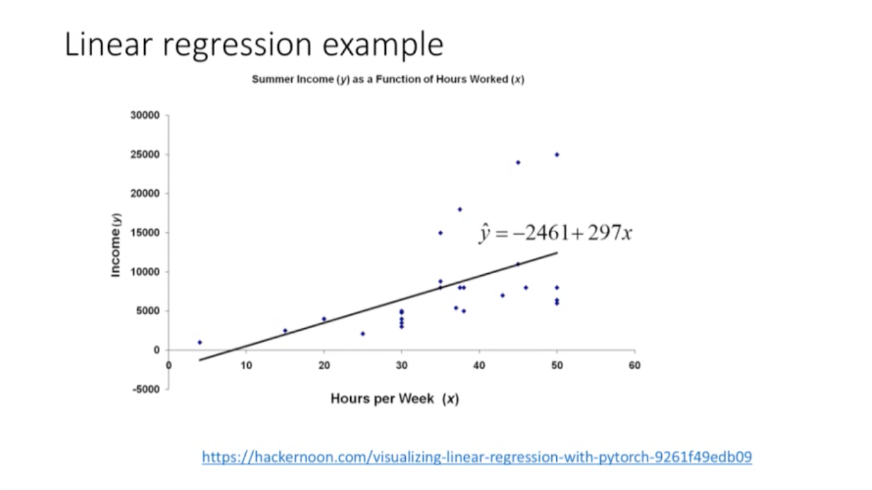
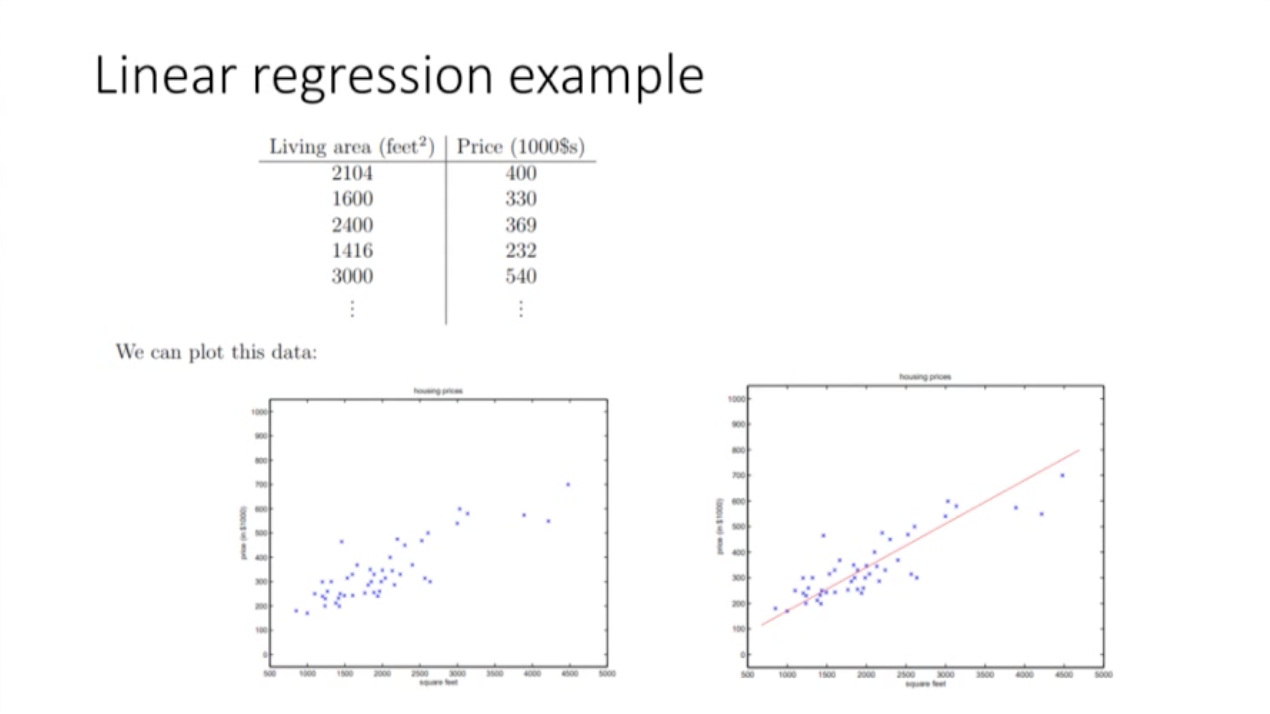

: 여러 직선을 그릴 수 있지만, 오차가 가장 적은 하나의 직선을 선택한다.

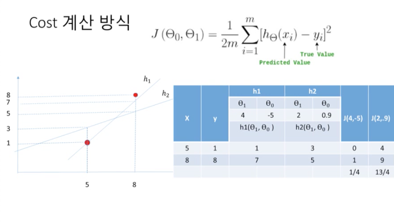
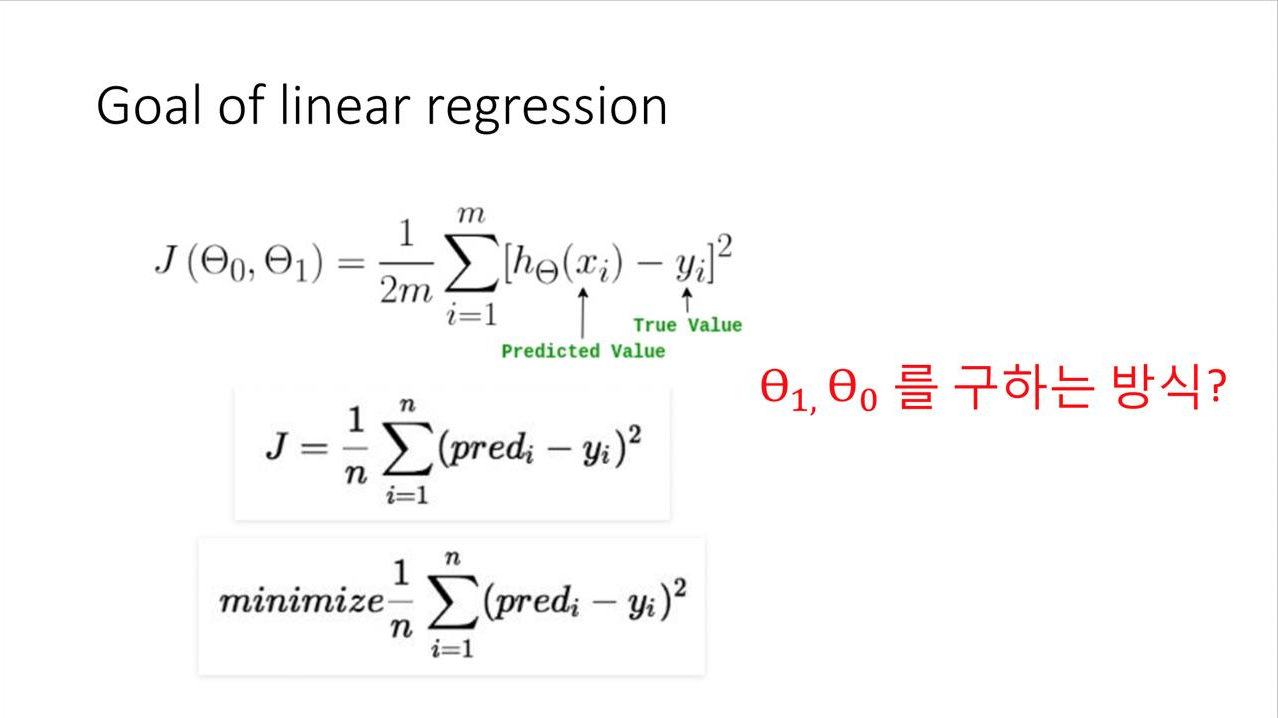
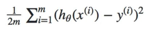
: m = 전체 데이터의 개수, y = 실제값, = 현재 세타에서 x_i에서의 예측값
: 오차의 제곱의 합을 구한 후, 평균을 구하면 cost가 된다.
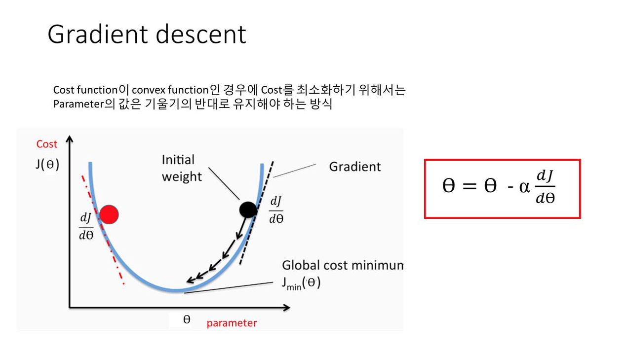
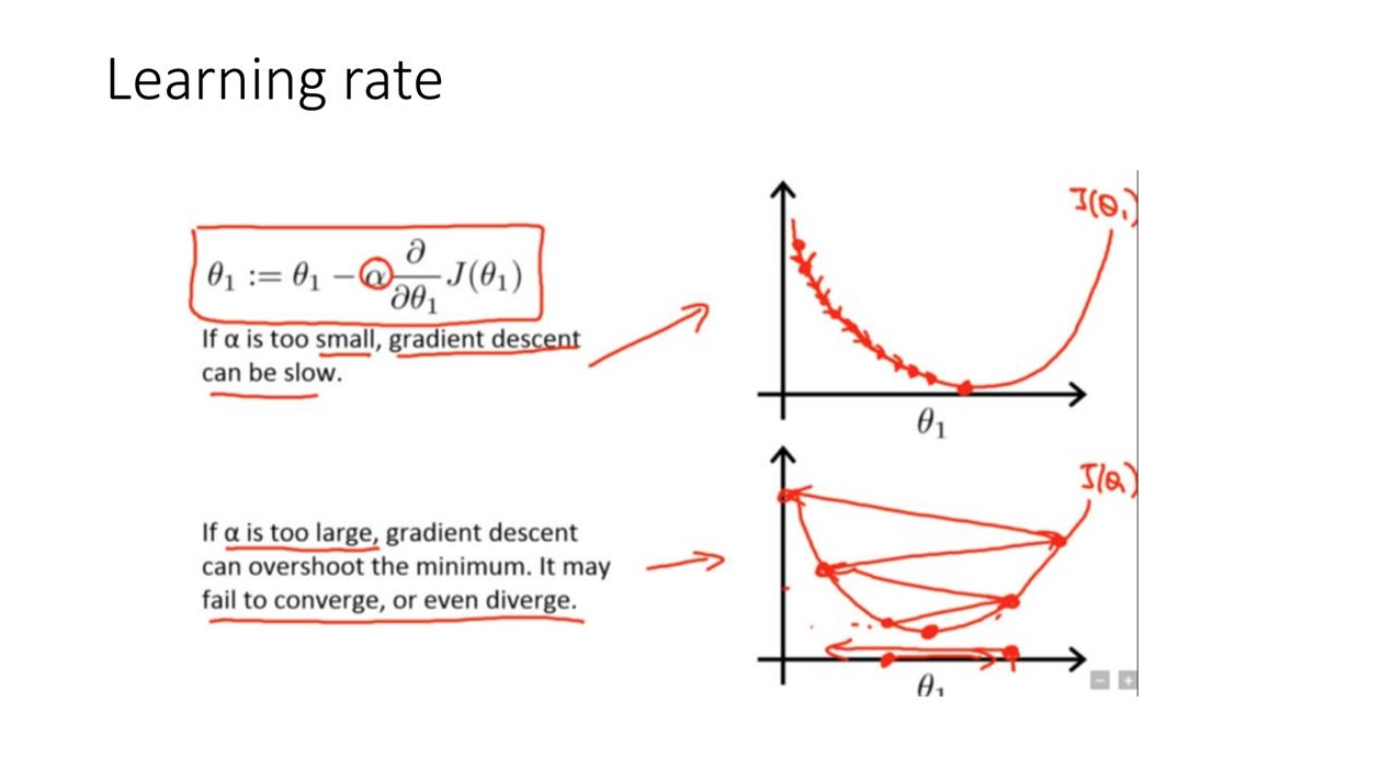
: 기울기의 반대 방향으로 조절하면서 적절한 값을 찾는다.


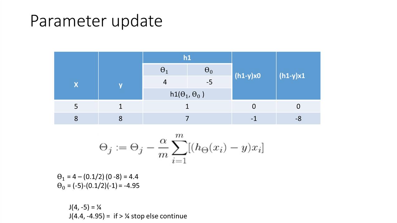
: x0 = 1 이라고 가정
코드
import numpy as np
import matplotlib.pyplot as plt
N = 500
X = 2 * np.random.rand(500,1)  #uniform distribution
y = 4 + 3 * X + np.random.randn(500, 1) #standard normal distributionprint(X.shape)
print(y.shape)
print(max(X))
print(min(X))
print(max(y))
print(min(y))(500, 1)
(500, 1)
[1.99953881]
[6.57142941e-05]
[11.70306469]
[2.02527574]plt.scatter(X,y)
# 500개의 데이터들이 표에 나타남<matplotlib.collections.PathCollection at 0x7fee748681d0>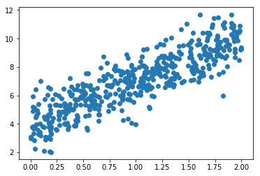
# 보기 편하게 설정
plt.figure(figsize = (10,10))
plt.scatter(X,y)
plt.title("Linear Regreesion Data")
plt.xlabel("x")
plt.ylabel("y")
plt.show()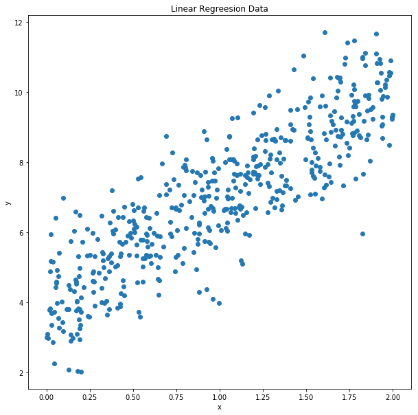
theta1 = 3
theta0 = 4
theta = np.array([[theta1, theta0]]).T
print(theta)
[[3]
[4]]oneColumns = np.full((N,1),1)
print(oneColumns.shape)
X1 = np.column_stack((X, oneColumns))
print(X1.shape)
print(X1[:10,:])(500, 1)
(500, 2)
[[1.85797371 1. ]
[1.29154213 1. ]
[0.557585 1. ]
[1.06541859 1. ]
[1.02518478 1. ]
[1.9769918 1. ]
[0.02221317 1. ]
[1.50834988 1. ]
[1.97880985 1. ]
[1.55130226 1. ]]predictions = X1 * Theta
X1.shape = (500,2), theta.shape = (2,1) 이므로, predictions 는 (500,1)
500개의 X에 대한 prediction
predictions = np.matmul(X1, theta) # 행렬 곱 실행predictions.shape(500, 1)plt.figure(figsize=(10,10))
plt.scatter(X,y)
plt.plot(X, predictions, color = "red")
plt.title("Linear Regression Data")
plt.xlabel("x")
plt.ylabel("y")
plt.show()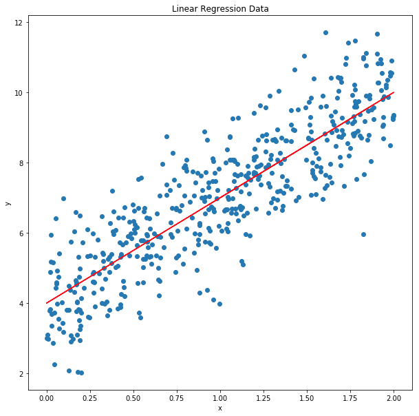
cost 계산
# Cost 계산
a = np.array([ [1],[2],[3] ])
b = np.array([ [2],[4],[1] ])
c = a - b
print(a)
print(b)
print(c)
d = np.square(c)
print(d)
print(np.sum(d))
[[1]
[2]
[3]]
[[2]
[4]
[1]]
[[-1]
[-2]
[ 2]]
[[1]
[4]
[4]]
9print(X1.shape)
print(X1.shape[0])
print(y.shape)
print(predictions.shape)
(500, 2)
500
(500, 1)
(500, 1)
def cost(X, y, theta):
m = X.shape[0]
predictions = np.matmul(X, theta)
diff = predictions - y
cost = (1/2*m)*np.sum(np.square(diff))
return costprint(cost(X1, y, theta))129436.48714975052theta update
x = np.array([ [10,1], [12,1], [20,1] ])
error = np.array([ [-1], [1],[2] ])
print(x)
print(error)
print(x.T)
delta = np.matmul(x.T, error)
print(delta)
[[10 1]
[12 1]
[20 1]]
[[-1]
[ 1]
[ 2]]
[[10 12 20]
[ 1 1 1]]
[[42]
[ 2]]a = np.array([ [10],[20] ])
print(a)
b = np.array([ [42],[2] ])
c = a - 0.4 * b
print(c)[[10]
[20]]
[[-6.8]
[19.2]]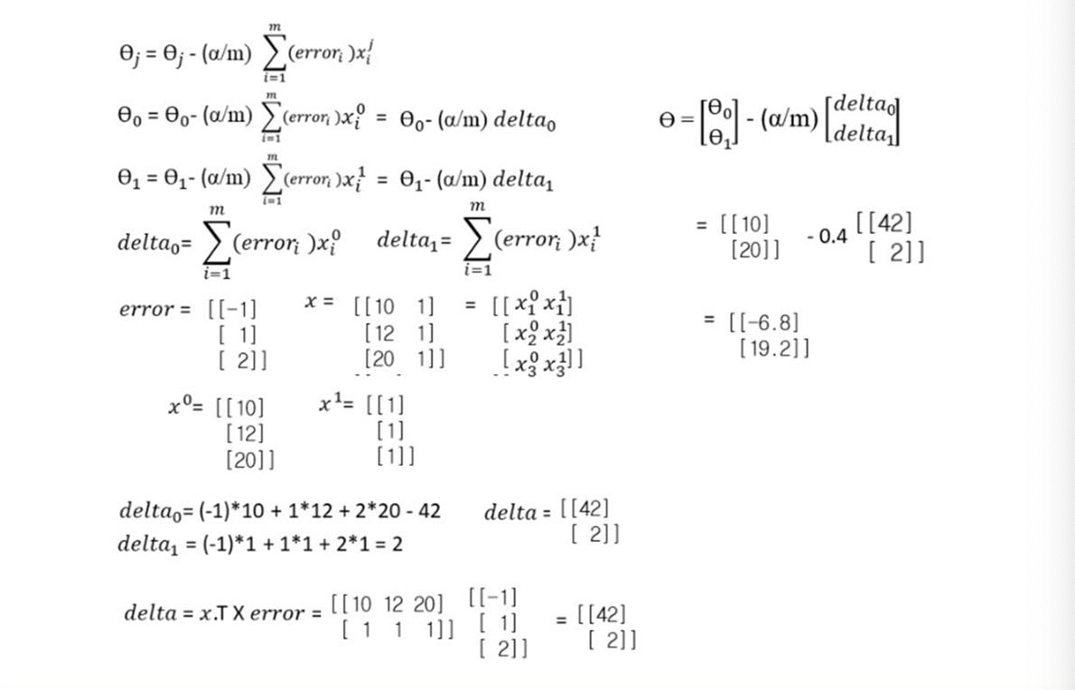
delta를 구해서 theta를 수정한다.
delta : x.T * error
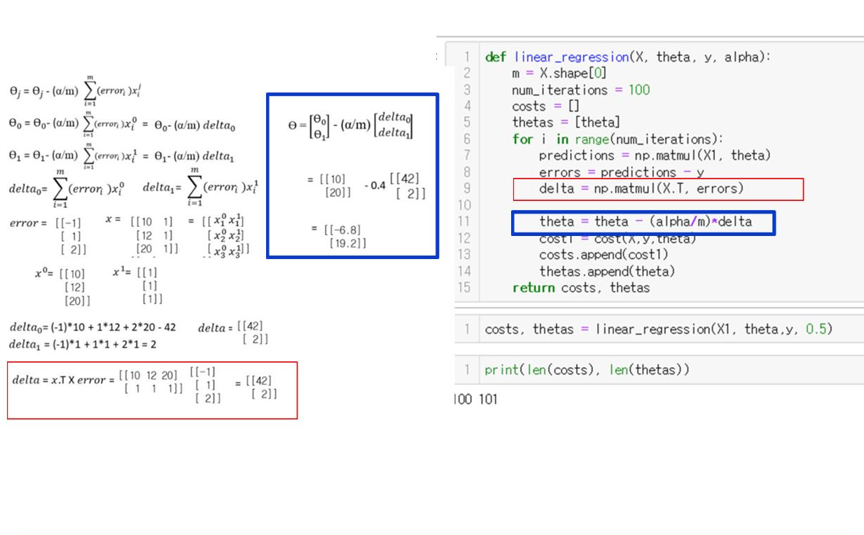
def linear_regression(X, theta, y, alpha):
    m = X.shape[0] # 데이터의 갯수
    num_iterations = 100
    costs = []
    thetas = [theta]
    for i in range(num_iterations):
        predictions = np.matmul(X1, theta)
        errors = predictions - y
        delta = np.matmul(X.T, errors)

        theta = theta - (alpha/m) * delta
        cost1 = cost(X,y,theta)
        costs.append(cost1)
        thetas.append(theta)
    return costs, thetas
theta1 = -5
theta0 = 5
theta = np.array([[theta1, theta0]]).T
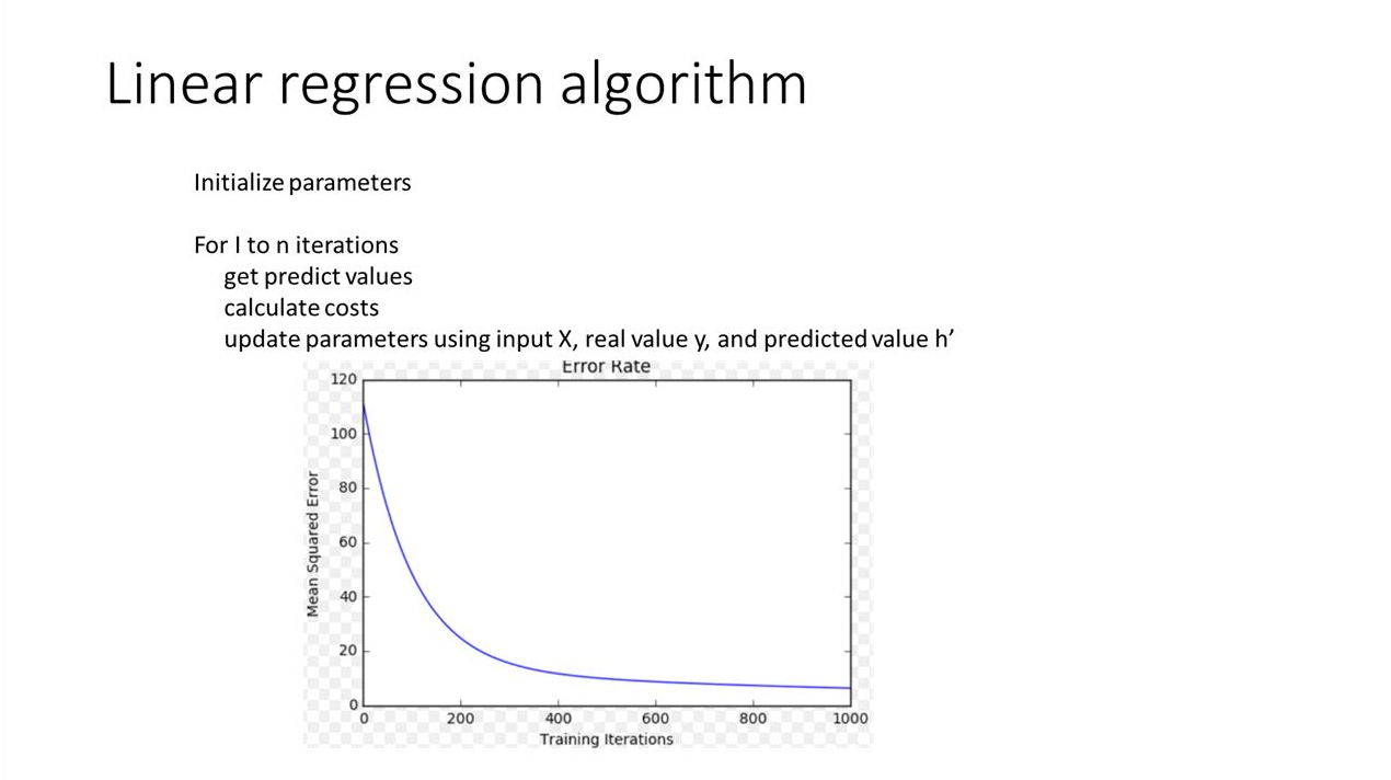
costs, thetas = linear_regression(X1, theta, y, 0.5)print(len(costs), len(thetas) )100 101plt.plot(costs) # cost가 점점 줄어드는 것을 볼 수 있다.[<matplotlib.lines.Line2D at 0x7fee77bf5470>]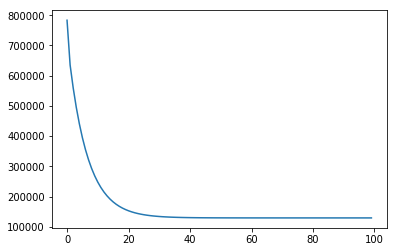
Initial and final regression
initialTheta = thetas[0] # 첫 세타 값
print(initialTheta)
finalTheta = thetas[-1] # 이터레이션이 충분히 이뤄진 개선된 세타
print(finalTheta)
prediction1 = np.matmul(X1, initialTheta)
prediction2 = np.matmul(X1, finalTheta)
[[-5]
[ 5]]
[[3.0549479 ]
[3.96520498]]plt.figure(figsize=(10,10))
plt.scatter(X, y)
plt.plot(X, prediction1, color="red")
plt.plot(X, prediction2, color="blue")
plt.title("Linear Regression Data")
plt.xlabel("x")
plt.ylabel("y")
plt.show()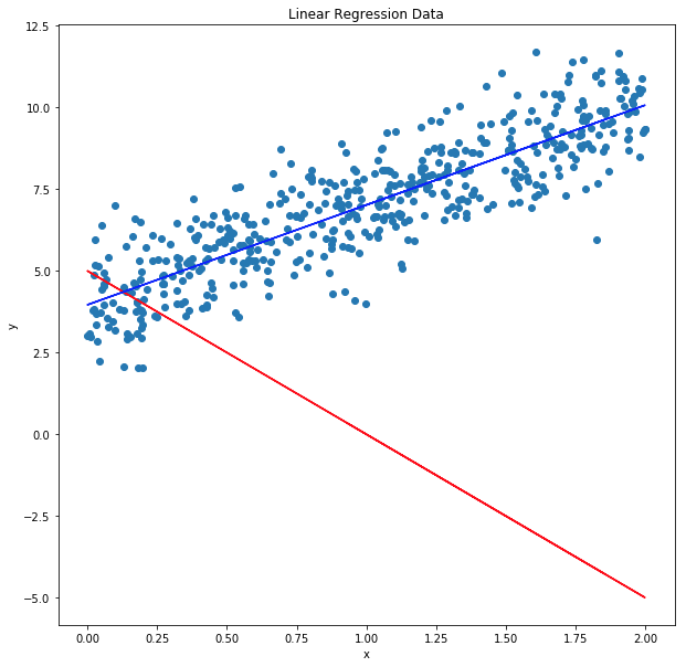

'당신을 한 줄로 소개해보세요'를 이 블로그로 대신 해볼까합니다.