Numpy

import numpy as np

List의 문제점

mathematical operations 부족, speed가 늦음

height = [170,180,170]
weight = [60,70,65]
weigth/height

---------------------------------------------------------------------------

TypeError                                 Traceback (most recent call last)

<ipython-input-11-38b806d7235c> in <module>
      1 height = [170,180,170]
      2 weight = [60,70,65]
----> 3 weigth/height


TypeError: unsupported operand type(s) for /: 'list' and 'list'

Solution : Numpy

1. Numeric Python
2. Alternative to python list : numpy Array
3. Calculations over entire arrays
4. Easy and fast

import numpy as np
np_height = np.array(height)
np_weight = np.array(weight)
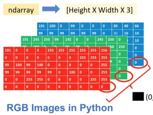
np_weight / np_height

array([0.35294118, 0.38888889, 0.38235294])

ndarray = N-dimensional array

print(type(np_weight))

<class 'numpy.ndarray'>

Numpy array creation

np.array([1,3,4,5])

array([1, 3, 4, 5])

data = [ [1,2], [11,22], [111,222] ]
a = np.array(data)
print(a)
print(type(a)) # numpyt 어레이로 만들면 타입이 ndarray 로 나옴

[[  1   2]
 [ 11  22]
 [111 222]]
<class 'numpy.ndarray'>

np.arange(10) ## vector 가 만들어짐

array([0, 1, 2, 3, 4, 5, 6, 7, 8, 9])

np.linspace(0,1,5) # 0~1까지 5등분을 한다. # 철자에 주의 line이 아니고 lin임

array([0.  , 0.25, 0.5 , 0.75, 1.  ])

Numpy arrays contain only one type

a = np.array([1.0, "is", True])
print(a)

['1.0' 'is' 'True']

Different use of + in Python and Numpy

python_list = [1,2,3]
np_list = np.array([1,2,3])
print(python_list + python_list)
print(np_list + np_list) # numpy의 경우 수학적 계산이 가능

[1, 2, 3, 1, 2, 3]
[2 4 6]

Numpy Subsetting

bmi = np.array([10,30,50,70])
print(bmi[2])
print(bmi > 35) # 35보다 큰 것들이 true가 되고 작은것들이 false가 되는 ndarray 리턴
print(bmi[bmi>35]) # 위에 연산에서 true 인 것들만 출력

50
[False False  True  True]
[50 70]

an_array = np.array( [[1,2,3,4,5] , [11,12,13,14,15]] )
print(an_array)
print(an_array[0])
print(an_array[0][2])
print(an_array[0,2])
print(an_array[:, 1:3]) #1~3까지 -> 1~2 인덱스 출력

[[ 1  2  3  4  5]
 [11 12 13 14 15]]
[1 2 3 4 5]
3
3
[[ 2  3]
 [12 13]]

Numpy Utilities

1. create a 2X2 array of zeros
2. create a 2X2 array filled with 9.0
3. create a 2X2 matrix with the diagonal 1s and th others 0
4. create a array of ones
5. create an array of random floats between 0 and 1

유틸리티들을 활용해서 다양한 기능을 구현할 수 있음

print(np.zeros((2,2)))  # zero로 채워진 매트릭스 생성
print(np.full((2,2), 9.)) # 원하는 수로 채워진 매트릭스 생성
print(np.eye(2,2)) # 대각선을 1로 채운 매트릭스
print(np.ones((2,2))) # 1로 채워진 매트릭스 생성
print(np.random.random((2,2))) # 0~1 사이의 랜덤 매트릭스 생성

[[0. 0.]
 [0. 0.]]
[[9. 9.]
 [9. 9.]]
[[1. 0.]
 [0. 1.]]
[[1. 1.]
 [1. 1.]]
[[0.09321367 0.76980373]
 [0.12700617 0.45380476]]

Numpy slicing

an_array = np.array([ [11,12,13,14], [21,22,23,24], [31,32,33,34] ])
print(an_array)

[[11 12 13 14]
 [21 22 23 24]
 [31 32 33 34]]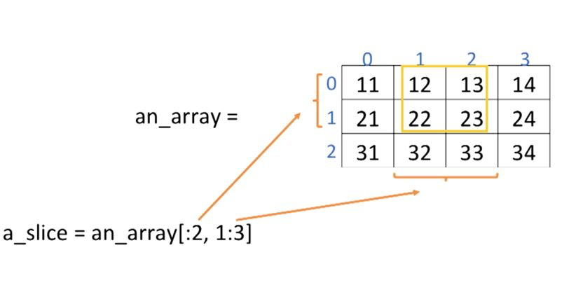

a_slice = an_array[:2, 1:3]
print(a_slice)

[[12 13]
 [22 23]]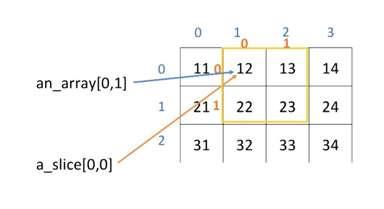

slice가 된 이후에는 인덱스가 새로 부여된다

슬라이스 인덱싱의 표현방법

Use arange and reshape to create an array in advance

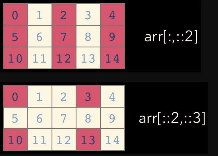
슬라이스 인덱싱의 표현방법
::2 -> 처음~끝, step:2 ::3 -> 처음~끝, step:3

a = np.arange(15)
print(a)
b = a.reshape(3,5) # ,로 구분 / 3행 5열의 매트릭스
print(b)
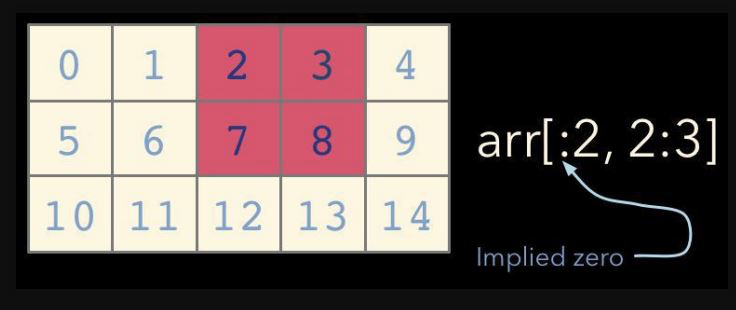
print(b[:2, 2:3]) # 행이 0~1까지 2개, 행은 2번째 인덱스 -> 결과로는 벡터가 아닌 매트릭스
print(a[0:5:2]) # a ndarray를 0~5까지 step 2로 인덱싱
print(a[::2]) 

[ 0  1  2  3  4  5  6  7  8  9 10 11 12 13 14]
[[ 0  1  2  3  4]
 [ 5  6  7  8  9]
 [10 11 12 13 14]]
[[2]
 [7]]
[0 2 4]
[ 0  2  4  6  8 10 12 14]

print(type(b))

<class 'numpy.ndarray'>

an_array = np.array([ [11,12,13,14], [21,22,23,24], [31,32,33,34] ])
a_slice = an_array[:2, 1:3]
print(a_slice)
print(an_array)
print("Before: ", an_array[0,1])
a_slice[0,0] = 1000
print("After : ", an_array[0,1])

#slice한 인덱스에서의 변화가 원래의 매트릭스에도 영향을 준다

[[12 13]
 [22 23]]
[[11 12 13 14]
 [21 22 23 24]
 [31 32 33 34]]
Before:  12
After :  1000

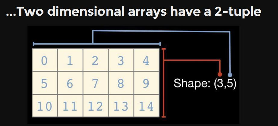
1-dimention : vector

2-dimention : matrix

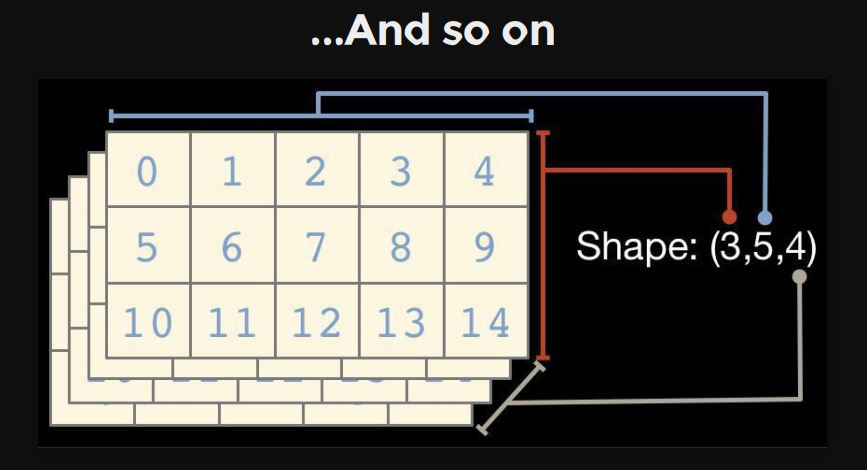
3-dimention : tensor

slice 된 것이 vector/matrix 인지 구분할 필요가 있음

슬라이싱 할때 특정한 로우나 컬럼([1]의 형태)을 지정하면 벡터가 나오고,
서브슬라이싱([1:2]의 형태)을 하게되면 매트릭스가 나온다.
[1]과 [1:2]는 같은 의미이지만 다른 타입을 리턴한다.

an_array = np.array([ [11,12,13,14], [21,22,23,24], [31,32,33,34]] )
print(an_array)
row_rank1 = an_array[1,:]
print(row_rank1, row_rank1.shape) # notice the shape : [] and vector

[[11 12 13 14]
 [21 22 23 24]
 [31 32 33 34]]
[21 22 23 24] (4,)

row_rank2 = an_array[1:2, :]
print(row_rank2, row_rank2.shape) # notice the shape : [[]] and matrix

[[21 22 23 24]] (1, 4)

# same thing can be done for columns of an array
col_rank1 = an_array[:, 1]
col_rank2 = an_array[:, 1:2]
print(col_rank1, col_rank1.shape, "-> vector")
print(col_rank2, col_rank2.shape, "-> matrix")

[12 22 32] (3,) -> vector
[[12]
 [22]
 [32]] (3, 1) -> matrix

an_array = np.array([ [11,12,13,14], [21,22,23,24], [31,32,33,34], [41,42,43,44] ])
print('Original Array:\n', an_array)
print(an_array.shape)

Original Array:
 [[11 12 13 14]
 [21 22 23 24]
 [31 32 33 34]
 [41 42 43 44]]
(4, 4)

# Use zip to generate coordinates
row_indices = np.arange(4)
col_indices = np.array([0,1,2,0])
print(row_indices)
print(col_indices)
print(zip(row_indices, col_indices))

[0 1 2 3]
[0 1 2 0]
<zip object at 0x7fbd99461d08>

for row, col in zip(row_indices, col_indices): # zip을 통해 두개의 vector를 합치다.
    print(row, " ", col)

0   0
1   1
2   2
3   0

print("Values: \n", an_array[row_indices, col_indices])

Values: 
 [11 22 33 41]

Boolean array 를 이용한 numpy array indexing

an_array = np.array([ [11,12], [21,22], [31,32] ])
filter = (an_array > 15) # The filter we've just created is the same size and shape
                         # as the original ndarray.
print(an_array)
print(filter)

[[11 12]
 [21 22]
 [31 32]]
[[False False]
 [ True  True]
 [ True  True]]

print(an_array[filter]) # true인 엘리민터를 찾아서 'vector'로 결과를 출력 
                        # matrix에서 vector로 결과가 바뀜

[21 22 31 32]

an_array[an_array > 15] # this is the same as above

array([21, 22, 31, 32])

an_array[(an_array > 20) & (an_array<30)] # 두개의 boolean array를 and연산도 가능

array([21, 22])

print(an_array[an_array % 2 == 0])
an_array[an_array % 2 == 0] += 100 # use similar filter to change elements
print(an_array)

[112 122 132]
[[ 11 212]
 [ 21 222]
 [ 31 232]]

a = np.arange(15).reshape((3,5))
print(a)
b = (a % 3 == 0)
print(b)
a[b]

[[ 0  1  2  3  4]
 [ 5  6  7  8  9]
 [10 11 12 13 14]]
[[ True False False  True False]
 [False  True False False  True]
 [False False  True False False]]





array([ 0,  3,  6,  9, 12])

Data type

ex1 = np.array([11,12]) # default로 데이터타입이 int로 지정됨
ex2 = np.array([11.0, 12.0]) # default로 데이터타입이 float으로 지정됨
ex3 = np.array([11,12], dtype=np.int64) # 데이터타입을 int로 지정
print(ex1.dtype)
print(ex2.dtype)
print(ex3.dtype)

int64
float64
int64

ex4 = np.array([11.1, 12.7], dtype=np.int64) # 데이터타입을 int로 지정
print(ex4)
print(ex4.dtype)
ex5 = np.array([11,12], dtype=np.float64) # 데이터타입을 float으로 지정
print(ex5)
print(ex5.dtype)

[11 12]
int64
[11. 12.]
float64

Arithmetic array operation

x = np.array( [[111,112], [121,122]] , dtype=np.int)
y = np.array( [[211.1, 212.1], [221.1, 222.2]], dtype=np.float64)
print(x + y)
print(np.add(x,y))

[[322.1 324.1]
 [342.1 344.2]]
[[322.1 324.1]
 [342.1 344.2]]

print(x-y)
print(np.subtract(x,y))

[[-100.1 -100.1]
 [-100.1 -100.2]]
[[-100.1 -100.1]
 [-100.1 -100.2]]

print(x/y)
print(np.divide(x,y))

[[0.52581715 0.52805281]
 [0.54726368 0.54905491]]
[[0.52581715 0.52805281]
 [0.54726368 0.54905491]]

print(np.sqrt(x))
print(np.exp(x))

[[10.53565375 10.58300524]
 [11.         11.04536102]]
[[1.60948707e+48 4.37503945e+48]
 [3.54513118e+52 9.63666567e+52]]

reshaping

# Change a shape
a = np.array(range(8))
print(a)
print(a.shape)
b = a.reshape((a.shape[0],1))
print(b)
print(b.shape)
c = a.reshape(2,4)
print(c)
d = a.reshape(2,2,2)
print(d)

[0 1 2 3 4 5 6 7]
(8,)
[[0]
 [1]
 [2]
 [3]
 [4]
 [5]
 [6]
 [7]]
(8, 1)
[[0 1 2 3]
 [4 5 6 7]]
[[[0 1]
  [2 3]]

 [[4 5]
  [6 7]]]

# "-1"을 활용하면 numpy가 shape를 알아서 결정
# "-1"는 한번만 사용 가능

b = np.arange(12).reshape(2,6)
print(b)
c = b.reshape(3,4)
print(c)
d = b.reshape(3,-1) # -1을 4로 치환해서 출력
print(d)

[[ 0  1  2  3  4  5]
 [ 6  7  8  9 10 11]]
[[ 0  1  2  3]
 [ 4  5  6  7]
 [ 8  9 10 11]]
[[ 0  1  2  3]
 [ 4  5  6  7]
 [ 8  9 10 11]]

Random number generation

arr = np.random.randn(2,5) # 평균 0, 표준편차 1 인 임의의 random 2 X 5 matrix
print(arr)
print("---0을 기준으로 표준편차가 1인 주변 값들이 랜덤으로 출력---\n")
arr = np.random.rand(2,5) # 0과 1 사이의 random number matrix
print(arr)
print("---0과 1사이의 무작위 값---\n")
arr = np.random.normal(50, .1, 5) # 평균 50, 표준편차 0.1, 갯수 5개
print(arr)
print("---갯수를 지정해서 vector 형식으로 출력---\n")

[[ 0.08802705  1.01537732  0.27631619  1.62960669  0.18818191]
 [ 0.21286143  0.01267762  2.01212436 -0.16928597 -1.37197614]]
---0을 기준으로 표준편차가 1인 주변 값들이 랜덤으로 출력---

[[0.17161559 0.33278003 0.64567763 0.88470556 0.1842044 ]
 [0.58886727 0.89425452 0.37286749 0.92839199 0.29320036]]
---0과 1사이의 무작위 값---

[50.16395078 50.03507731 49.96453089 50.0416792  50.06299656]
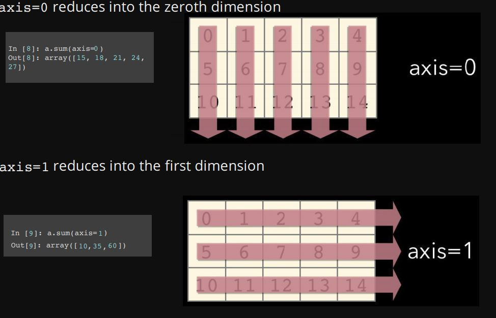
---갯수를 지정해서 vector 형식으로 출력---

numpy axis

axis=0 는 컬럼으로 합침
(0번째 인덱스인 3이 1으로 바뀐다고 생각하면 쉬움)

arr = np.random.randn(2,5) # 평균 0, 표준편차 1 인 임의의 random 2 X 5 matrix
print(arr)
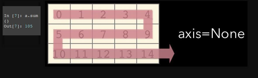
# compute mean for all elements
print(arr.mean())
# compute the means by row
print(arr.mean(axis = 1))
# compute the means by column
print(arr.mean(axis = 0))

[[-1.01849505  0.44179238 -0.89571664  0.62823837 -0.34392035]
 [-0.44528444  1.63285507  0.28823175  1.458288    0.96866307]]
0.27146521628240355
[-0.23762026  0.78055069]
[-0.73188974  1.03732372 -0.30374244  1.04326319  0.31237136]

Sorting and set operations

unsorted = np.random.randn(10)
print(unsorted)

[ 0.89700477  1.25200837  1.14901376  0.47956963 -0.25656664  0.40453951
  0.68525313 -1.5086035  -1.0621123  -1.13511072]

# create copy and sort
sorted = np.array(unsorted)
sorted.sort()
print(sorted)

[-1.5086035  -1.13511072 -1.0621123  -0.25656664  0.40453951  0.47956963
  0.68525313  0.89700477  1.14901376  1.25200837]

# finding unique elements
array = np.array([1,2,3,1,2,3])
np.unique(array) # 중복된 엘리먼트를 제외하고 출력

array([1, 2, 3])

# set operation
s1 = np.array(["desk", "chair", "bulb"])
s2 = np.array(["lamp", "bulb", "chair"])

#operation 이름에 1d를 붙여 사용
print(np.intersect1d(s1, s2)) # s1와 s3의 교집합
print(np.union1d(s1, s2)) # s1와 s2의 합집합
print(np.setdiff1d(s1,s2)) # s1 기준 s2와의 차집합
print(np.in1d(s1, s2)) # which element of s1 in also in s2

['bulb' 'chair']
['bulb' 'chair' 'desk' 'lamp']
['desk']
[False  True  True]

Broadcasting

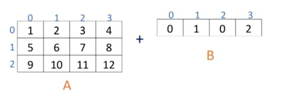
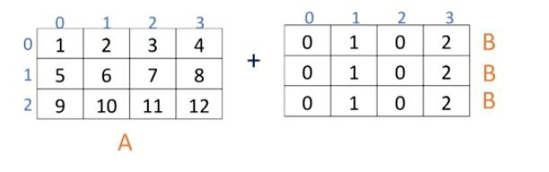
부족한 행, 열을 자동으로 맞춰준다

# introduction in broadcasting

start = np.zeros((4,3))
add_rows = np.array([1,0,2])
print(start)
print(add_rows)

[[0. 0. 0.]
 [0. 0. 0.]
 [0. 0. 0.]
 [0. 0. 0.]]
[1 0 2]

# use broadcast to add to each row of 'start'
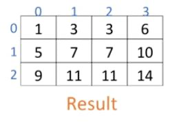
y = start + add_rows
print(y)

[[1. 0. 2.]
 [1. 0. 2.]
 [1. 0. 2.]
 [1. 0. 2.]]

add_cols = np.array([[0,1,2,3]]) # notice [[ ]] not [ ], transform하기 위해서
add_cols = add_cols.T # transform 
print(add_cols)
y = start + add_cols
print(y)

[[0]
 [1]
 [2]
 [3]]
[[0. 0. 0.]
 [1. 1. 1.]
 [2. 2. 2.]
 [3. 3. 3.]]

add_scalar = np.array([1])
print(add_scalar)
# It's worth showing that our addition of a scalar value
# like one, to start works fine,
# as it will broadcast in both directions.
print(start + add_scalar) # 행열을 자동을 늘려서 더해줌

[1]
[[1. 1. 1.]
 [1. 1. 1.]
 [1. 1. 1.]
 [1. 1. 1.]]

Application

%matplotlib inline
from scipy import misc
import matplotlib.pyplot as plt
# from skimage import data
photo_data = misc.imread('/Users/isanghyeon/Downloads/6.1 numpy/sd-3layers.jpg')
type(photo_data)

/Users/isanghyeon/anaconda3/lib/python3.6/site-packages/ipykernel_launcher.py:5: DeprecationWarning: `imread` is deprecated!
`imread` is deprecated in SciPy 1.0.0, and will be removed in 1.2.0.
Use ``imageio.imread`` instead.
  """





numpy.ndarray

# Let's see what is in the image
plt.figure(figsize=(15,15))
plt.imshow(photo_data)

<matplotlib.image.AxesImage at 0x7fbd9cab5ba8>

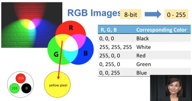
print(photo_data.shape)

(3725, 4797, 3)

photo_data.size

53606475

photo_data.max(), photo_data.min(), photo_data.mean()

(255, 0, 75.8299354508947)

#Pixel on the 150th row and 250th column
photo_data[150,200], photo_data[150,200,1]

(array([17, 55, 94], dtype=uint8), 55)

photo_data[200:800, : , 1] = 255 # green값을 최대로
plt.figure(figsize = (10,10))
plt.imshow(photo_data)

<matplotlib.image.AxesImage at 0x7fbd796fcc18>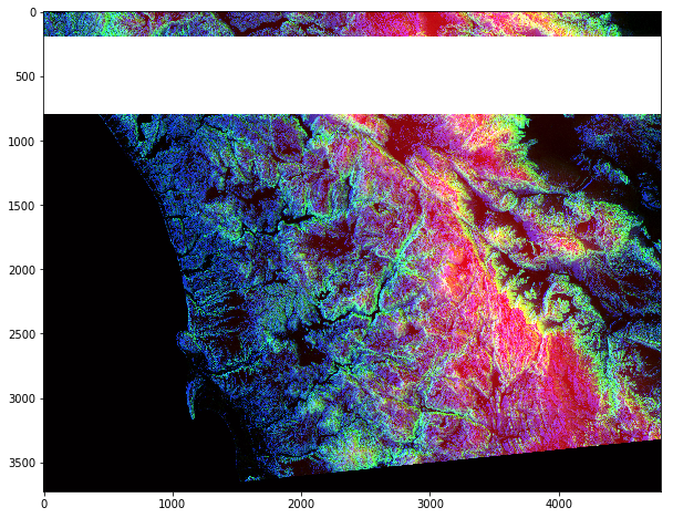

photo_data[200:800, :] = 255
plt.figure(figsize = (10,10))
plt.imshow(photo_data)

<matplotlib.image.AxesImage at 0x7fbd79a094a8>

photo_data[200:800, :] = 0
plt.figure(figsize=(10,10))
plt.imshow(photo_data)

<matplotlib.image.AxesImage at 0x7fbd811b0438>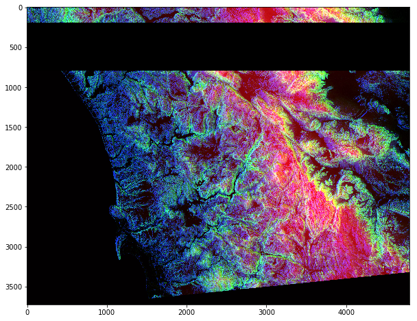

photo_data = misc.imread('/Users/isanghyeon/Downloads/6.1 numpy/sd-3layers.jpg')
print(photo_data.shape) # x,y,rgb 로 구성
low_value_filter = photo_data < 100
print(low_value_filter.shape) # rgb 값이 100보다 작은 부분의 boolean벡터 생성
print(photo_data[0][0])
print(photo_data[100][100])
print(low_value_filter[0][0])
print(low_value_filter[100][100])

/Users/isanghyeon/anaconda3/lib/python3.6/site-packages/ipykernel_launcher.py:1: DeprecationWarning: `imread` is deprecated!
`imread` is deprecated in SciPy 1.0.0, and will be removed in 1.2.0.
Use ``imageio.imread`` instead.
  """Entry point for launching an IPython kernel.


(3725, 4797, 3)
(3725, 4797, 3)
[ 0 22 35]
[ 39 143 156]
[ True  True  True]
[ True False False]

plt.figure(figsize = (10,10))
plt.imshow(photo_data)
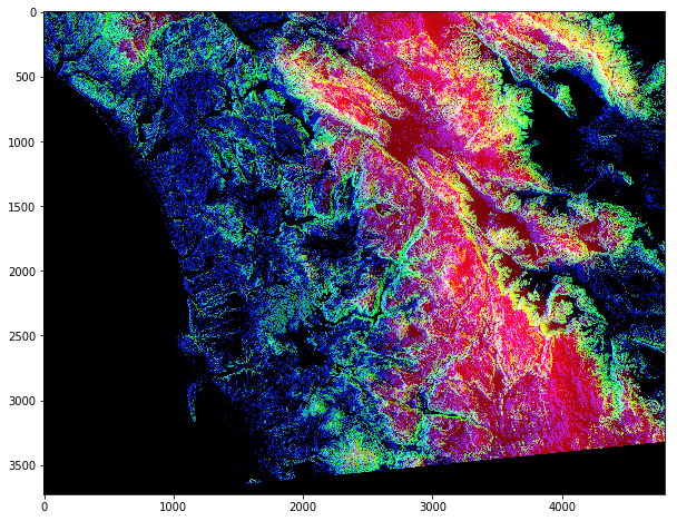
photo_data[low_value_filter] = 0
plt.figure(figsize = (10,10))
plt.imshow(photo_data)

## 결과적으로 rgb값 중 100보다 작은 rgb를 filter해서 이미지를 처리함

<matplotlib.image.AxesImage at 0x7fbd5932bbe0>