A Neural Network Playground - TensorFlow : https://bit.ly/487HdL1
Chapter 7. 성능 관리
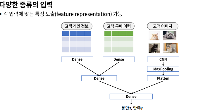
적절한 모델
- 모델마다 각각 복잡도 조절 방법이 존재
- 복잡도를 조금씩 조절해가면서 (하이퍼파라미터 조정) train eroor와 validation error을 측정하고 비교. (관점은 validation error)
딥러닝에서 조절할 대상
- epoch 와 learning_rate
- 모델 구조 : hidden layer수 , node 수
- 미리 멈춤 Early Stopping
- 임의 연결 끊기 Dropout
- 가중치 규제하기 Regularization(L1,L2)
딥러닝 복잡도 : hidden layer 수, node 수
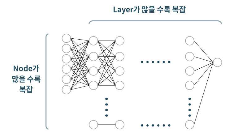
- 딥러닝 모델의 복잡도 혹은 규모와 관련된 수 : 파라미터(가중치) 수
- Input feature 수, hidden layer 수, node 수와 관련있음
- Conv Layer 인 경우, MaxPooling Layer를 거치면서 데이터가 줄어들어 파라미터 수 감소
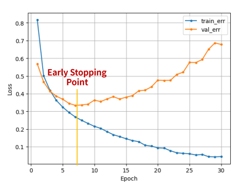
미리 멈춤 Early Stopping
-
반복(epoch)가 많으면 과적합 될 수 있음
- 항상 과적합이 발생되는 것은 아님
- 반복횟수가 증가할 수록 val error가 줄어들다가 어느 순간 증가할 수 있음
-
val error가 더이상 줄 지 않으면 멈춰라 : Early Stopping
-
일반적으로 train error는 계속 줄어 듦
-
Early stopping 옵션
- monitor : 기본값 val_loss
- min_delta : 오차(loss)의 최소값에서 변화량이 몇 이상 되어야 하는지 지정 (기본값 0)
- patience : 오차가 줄어들지 않는 상황을 몇번(epoch) 기다려 줄건지 지정 (기본값 0)
from keras.callbacks import EarlyStopping
es = EarlyStopping(monitor = 'val_loss', min_delta = 0, patience = 0)- .fit(,,,callbacks=[es]) : epoch단위로 학습이 진행되는 동안, 중간에 개입할 task 지정
model.fit(x_train, y_train, epochs = 100, validation_split = .2, callbacks = [es])연결을 임의로 끊기 Dropout
-
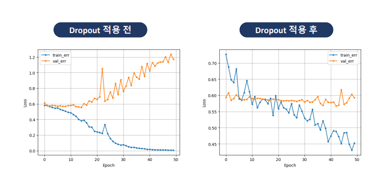
과적합을 줄이기 위해 사용되는 규제regularization 기법 중 하나
-
학습시, 신경망의 일부 뉴런을 읨이로 비활성화 -> 모델을 강제로 일반화
-
절차
- 훈련 배치에서 랜덤하게 선택된 일부 뉴런을 제거
- 제거된 뉴런은 해당 배치에 대한 순전파 및 역전파 과정에서 비활성화
- 이를 통해 뉴런들 간의 복잡한 의존성을 줄여줌
- 매 epochs마다 다른 부분 집합의 뉴런을 비활성화 -> 앙상블 효과
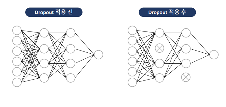
- Hidden Layer 다음에 Dropout Layer 추가
# hidden layer 노드 중 40%를 임의로 제외 시킴
# 보통 0.2~0.5 사이의 범위 지정
model3 = Sequential( [Input(shape = (nfeatures,)),
                      Dense(128, activation= 'relu'),
                      Dropout(0.4),
                      Dense(64, activation= 'relu'),
                      Dropout(0.4),
                      Dense(32, activation= 'relu'),
                      Dropout(0.4),
                      Dense(1, activation= 'sigmoid')] )
모델 저장하기 : 최종 모델 저장하기
model.save('파일이름.keras')- 모델 로딩하기
from keras.models import load_model
model2 = load_model('파일이름.keras')
모델 저장하기 : 중간 체크포인트 저장하기
from keras.callbacks import ModelCheckpoint

cp_path = '/content/{epoch:03d}.keras'  # Keras 2.11 이상 버전에서 모델 확장자 .keras
mcp = ModelCheckpoint(cp_path, monitor='val_loss', verbose = 1, save_best_only=True)

# 학습
hist = model1.fit(x_train, y_train, epochs = 50, validation_split=.2, callbacks=[mcp]).history- save_best_only=True : 이전 체크 포인트의 모델들 보다 성능이 개선되면 저장
Chapter 8. Functional API
Funtional
- 연결될 앞 레이어 지정
- Model()함수로 시작과 끝을 연결해서 선언
clear_session()

il = Input(shape=(nfeatures, ))
hl1 = Dense(18, activation='relu')(il)
hl2 = Dense(4, activation='relu')(hl1)
ol = Dense(1)(hl2)

model = Model(inputs = il, outputs = ol)

model.summary()
다중 입력
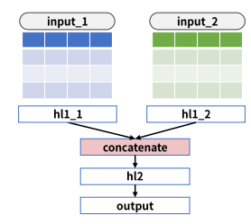
# 모델 구성
# name 은 생략 가능
input_1 = Input(shape=(nfeatures1,), name='input_1')
input_2 = Input(shape=(nfeatures2,), name='input_2')

# 첫 번째 입력을 위한 레이어
hl1_1 = Dense(10, activation='relu')(input_1)

# 두 번째 입력을 위한 레이어
hl1_2 = Dense(20, activation='relu')(input_2)

# 두 히든레이어 결합 (리스트로)
cbl = concatenate([hl1_1, hl1_2])

# 추가 히든레이어
hl2 = Dense(8, activation='relu')(cbl)

# 출력 레이어
output = Dense(1)(hl2)

# 모델 선언(리스트)
model = Model(inputs = [input_1, input_2], outputs = output)

model.summary()- 모델 학습,예측시에도 리스트 활용
# 학습
hist = model.fit([x_train1, x_train2], y_train, epochs=50, validation_split=.2).history

#예측
pred = model.predict([x_val1, x_val2])
Chapter 9. 시계열 모델링 기초
- Sequential + 시간의 등 간격
- 시간의 흐름에 따른 패턴을 분석
- 흐름을 어떻게 정리할 것인지에 따라 모델링 방식이 달라짐
Modeling - 통계적 시계열 모델링
- y의 이전 시점 데이터들로 흐름의 패턴을 추출하여 예측
- 패턴 : Trand, Seasonality
- X 변수들은 사용하지 않음
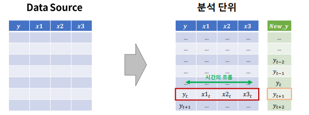
Modeling - ML기반 시계열 모델링
- 특정 시점 데이터들(1차원)과 예측대상시점과의 관계로 부터 패턴을 추출하여 예측
- 시간의 흐름을 X 변수로 도출하는 것이 중요
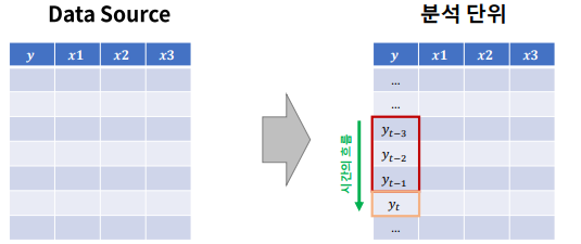
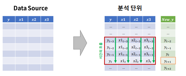
Modeling - DL 기반 시계열 모델링
- 시간 흐름 구간(timesteps) 데이터들(2차원) 과 예측 대상 시점과의 관계로 부터 패턴을 추출
- 어느 구간을 하나의 단위로 정할 것인가?
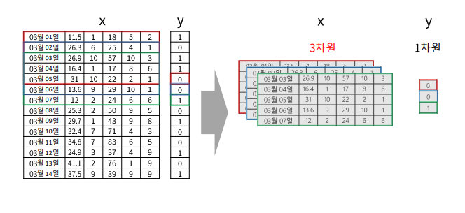
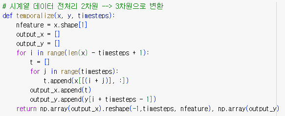
- 분석 단위를 2차원으로 만드는 전처리 필요 -> 데이터 셋은 3차원
시계열 모델링 절차
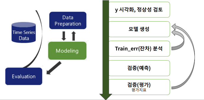
RNN(Recurrent Neural Networks)으로 시계열 데이터 모델링 하기
- 과거의 정보를 현재에 반영해 학습하도록 설계
<절차>
1. 데이터 분할 1:x,y
2. 스케일링
- X스케일링은 필수
- Y값이 크다면 최적화를 위해 스케일링 필요 -> 단, 모델 평가 싱 원래 값으로 복원
- 3차원 데이터셋 만들기
- 데이터 분할2:train, val
3. 3차원 데이터 셋 만들기
2차원 데이터셋(X) -> timesteps 단위로 잘라서
(한칸 씩 밀면서)
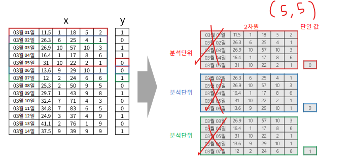
- 3차원 구조 생성
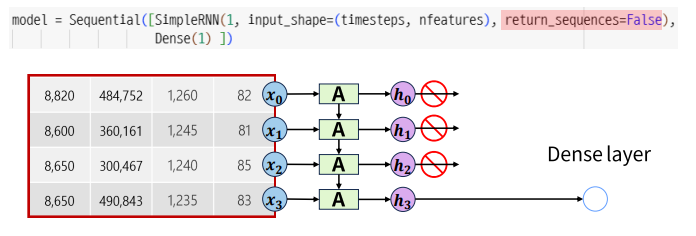
SimpleRNN Layer 1개
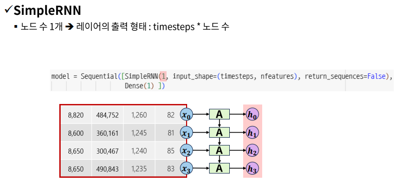
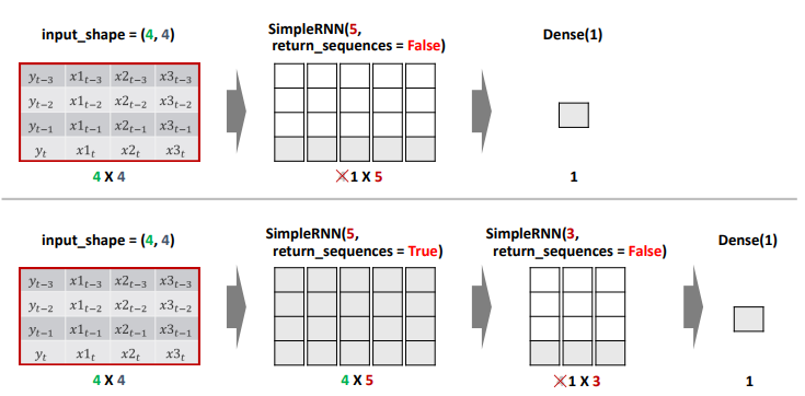
- return_sequences : 출력 데이터를 다음 레이어에 전달할 크기 결정
- True : 출력 크기 그대로 전달 -> timestemps*node수
- False(default) : 가장 마지막(최근) hidden state 값만 전달 -> 1*node수
SimpleRNN Layer 여러개
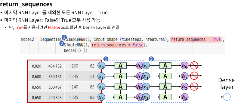
+) 만약 RNN Layer을 중첩해서 hidden layer을 만들려면,
마지막 output layer 바로 전이 아닌이상, return_sequences =True 로 시계열을 유지하여 넘겨야 한다.
시계열 모델링 실습 :서울의 주간평균기온
- 데이터 준비
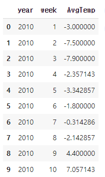
1)🌟 y 만들기
data['y'] = data['AvgTemp'].shift(-1)
data.dropna(axis = 0, inplace = True)
data.head()
2) x,y 분리
x = data.loc[:, ['AvgTemp']]
y = data.loc[:,'y']
3) 스케일링
scaler = MinMaxScaler()
x = scaler.fit_transform(x)
4) 🌟3차원 구조 만들기
# 4주간의 데이터가 한 단위
x2, y2 = temporalize(x, y, 4)
x2.shape, y2.shape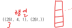
5) 데이터 분할
# shuffle=False : 랜덤 분할하지 마라
# test_size = 숫자 : 데이터 건수 (끝에서부터)
# 53은 1년치 데이터
x_train, x_val, y_train, y_val = train_test_split(x2, y2, test_size= 53, shuffle = False)- RNN 모델링
1) 🌟입력 구조 (shape)
# 분석 단위 2차원 (timesteps, nefeatures)
timesteps = x_train.shape[1]
nfeatures = x_train.shape[2]
2) 🌟모델 구조 설계
- SimpleRNN(8, input_shape = (timesteps, nfeatures))
- Dense(1)
clear_session()

model = Sequential([Input(shape = (timesteps, nfeatures)),
                    SimpleRNN(8), # 4*8
                    Dense(1)]) # 1

model.summary()
3) 컴파일 및 학습
model.compile(optimizer = Adam(0.01), loss = 'mse')
hist = model.fit(x_train, y_train, epochs = 100, verbose = 0, validation_split = .2).history
4) 예측 및 평가
# 예측
pred = model.predict(x_val)

# 평가
mean_absolute_error(y_val, pred)
5) 시각화
plt.figure(figsize = (10,6))
plt.plot(y_val, label = 'actual')
plt.plot(pred, label = 'predicted')
plt.legend()
plt.grid()
plt.show()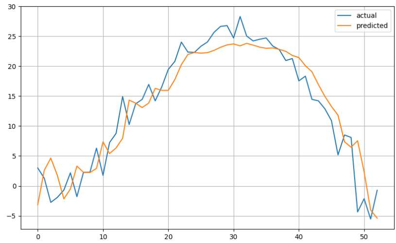
LSTM (Long Short-Term Meory)
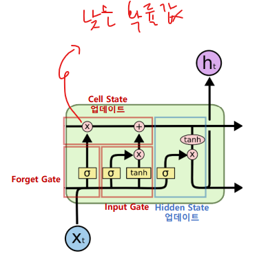
LSTM 구조 : time step 간에 두 종류의 상태 값 업데이트 관리
- Hidden State 업데이트
- Cell State 업데이트 : 긴 시퀀스 동안 정보를 보존하기 위한 상태 값이 추가됨
- forget Gate
- Input Gate
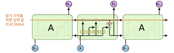
- Cell State 업데이트
- 불필요한 과거는 잊어라(Forget Gate)
- 현재 정보 중 중요한 것은 기억하라 (Input Gate)
- Inpute Gate 와 Forget Gate를 결합해서 장기 기억 메모리에 태워라 (cell state 업데이트)
- Hidden State 업데이트
- [업데이트된 cell state]와 [input, 이전셀의 hidden state] 으로 새 hidden state 값 생성해서 넘기기

복습 복습 복습