DCGAN 모델 구현
Pytorch를 이용하여 DCGAN을 구현한다. DCGAN은 Deep Convolutional Generative Adversarial Network의 약자로, Generator와 Discriminator에서 Fully connected layer가 아닌 Convolutional layer를 사용하는 모델이다. CNN의 특성으로 인해 공간적 정보를 더 잘 학습하여 DCGAN으로 만들어진 latent vector(noise)는 이미지의 연속성을 더 잘 표현할 수 있다.
데이터셋은 CelebA 데이터셋을 사용할 것이다. 데이터셋에 관한 정보는 아래 링크에서 자세히 확인할 수 있다.
https://www.kaggle.com/datasets/jessicali9530/celeba-dataset
우리의 목적은 Generative Model 구현이기 때문에 CelebA 데이터셋에서 이미지 데이터만을 사용할 것이다.
Import
필요한 것들을 import 해준다.
import random

import torch
import torch.nn as nn
import torch.nn.parallel
import torch.utils.data
import torchvision
import torchvision.datasets as dataset
import torchvision.transforms as transforms

import numpy as np

import matplotlib.pyplot as plt
import matplotlib.gridspec as gridspec
%matplotlib inline
Dataset
데이터셋을 불러오기 전에 필요한 변수들을 정의해준다.
PATH = './celebA/'

batch_size = 128

img_size = 64

z_size = 100

epochs = 8

learning_rate = 0.0002

# Beta1 hyperparameter(for Adam)
beta1 = 0.5

real_label = 1
fake_label = 0
이제 데이터셋을 불러올 것인데, Dataset의 shape가 (178 X 218) 이므로 torchvision.transforms을 이용하여 데이터셋을 불러온 이후에 img_size(=64)만큼 Resize, crop 하고, 텐서화 한 다음에 Normalization 해준다.
transform = transforms.Compose([
    transforms.Resize(img_size),
    transforms.CenterCrop(img_size),
    transforms.ToTensor(),
    transforms.Normalize((0.5, 0.5, 0.5), (0.5, 0.5, 0.5))])

img_dataset = dataset.ImageFolder(root=PATH,
                           transform=transform)

data_loader = torch.utils.data.DataLoader(dataset=img_dataset,
                                           batch_size=batch_size,
                                           shuffle=True,
                                           drop_last=True)
Dataset Preview
def imgshow(inp, title=None):
inp = inp.numpy().transpose((1, 2, 0))
mean = np.array([0.5, 0.5, 0.5])
std = np.array([0.5, 0.5, 0.5])
inp = std * inp + mean
inp = np.clip(inp, 0, 1)
plt.imshow(inp)
if title is not None:
plt.title(title)
plt.pause(0.001)
for i in range(4):
sample_data_loader = torch.utils.data.DataLoader(dataset=img_dataset,
batch_size=4,
shuffle=True)
inputs, classes = next(iter(sample_data_loader))
out = torchvision.utils.make_grid(inputs)
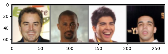
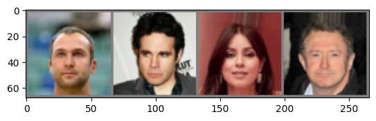
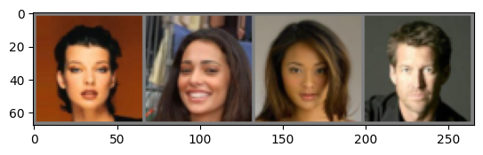
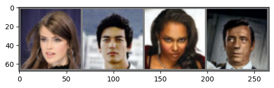
imgshow(out)해당 함수를 구현하여 데이터셋을 미리 preview 할 수 있다.
임시적인 sample_data_loader를 통해 batch size를 4로 정해주고, for문을 이용하여 4개의 batch를 확인할 수 있다.
Model 구현 & 정의
Generator와 Discriminator를 정의할 것이다.
두 모델 모두 FCN, Pooling layer를 사용하지 않고, 마지막 layer를 제외한 모든 layer에 nn.BatchNorm2d를 이용하여 Batch Normalization을 적용할 것이다. 또한 이전 포스팅과 마찬가지로 xavier 초기화를 사용한다.
nn.BatchNorm2d에 대한 간략한 설명은 아래와 같다.
nn.BatchNorm2d
nn.BatchNorm2d를 이용하면 말 그대로 2차원 이미지 데이터에 대한 Batch Normalization을 수행할 수 있다.
# num_features를 제외한 모든 변수들은 Default값을 기술함
nn.BatchNorm2d(num_features, eps=1e-05, momentum=0.1, affine=True, track_running_stats=True)
num_features: 입력 채널의 개수
eps: 분모에 더해지는 값(매우 작음)
momentum: Batch Normalization의 Running mean 과 Running variance를 계산할 때 사용되는 값
affine: Affine parameter들을 학습할지에 대한 여부
track_running_stats: Batch Normalization의 통계량을 추적할지에 대한 여부
Generator에는 nn.ConvTranspose2d를 이용하여 Transposed convolution 연산을 수행할 것인데, 이에 대한 간단한 설명도 아래에 서술하겠다.
Transposed convolution
Transposed convolution 연산은 Convolution 연산과 반대로 upsampling을 수행할 수 있다. 즉, input data에 비해 output data의 차원이 커지게 된다. nn.ConvTranspose2d를 통해 Transposed convolution 연산을 수행할 수 있는데, 이는 Semantic Segmentation에 자주 사용된다.
Semantic Segmentation 작업에서는 Downsamping(Encoder) 과정을 통해 이미지의 특징을 추출하고, 그 후 upsampling(Decoder) 과정을 통해 본래의 이미지 크기로 복원하여 이미지의 모든 픽셀들을 분류할 수 있게 된다. 이 upsampling 과정에서 사용되는 것이 nn.ConvTranspose2d이다.
nn.ConvTranspose2d도 nn.Conv2d처럼 kernel, stride, padding과 같은 parameter들을 이용하는 것은 같다. 하지만 연산과정에서는 약간의 차이가 있다.
만약 input data의 shape가 (2, 2, 1), kernel의 shape가 (3, 3, 1), stride = 1, padding = 1 인 경우의 연산의 양상은 아래와 같다.
 초록색은 output data이고, 파란색은 input data이다.
이와 같이 output data의 크기가 input data에 비해 증가하게 된다.
output data의 한 변의 크기를 구하는 공식은 아래와 같다.
input data의 크기:
output data의 크기:
kernel의 크기:
stride:
padding:
이제 본격적으로 모델을 구현해보겠다.
class Generator(nn.Module):
    def __init__(self):
        super(Generator, self).__init__()

        self.upconv1 = nn.Sequential(
            nn.ConvTranspose2d(
                in_channels=z_size,
                out_channels=512,
                kernel_size=(4, 4),
                stride=(1, 1),
                bias=False
                ),
            nn.BatchNorm2d(
                num_features=512,
                eps=1e-05,
                momentum=0.1,
                affine=True,
                track_running_stats=True
                ),
            nn.ReLU(inplace=True)
        )
        self.upconv2 = nn.Sequential(
            nn.ConvTranspose2d(
                in_channels=512,
                out_channels=256,
                kernel_size=(4, 4),
                stride=(2, 2),
                padding=(1, 1),
                bias=False
                ),
            nn.BatchNorm2d(
                num_features=256,
                eps=1e-05,
                momentum=0.1,
                affine=True,
                track_running_stats=True
                ),
            nn.ReLU(inplace=True)
        )
        self.upconv3 = nn.Sequential(
            nn.ConvTranspose2d(
                in_channels=256,
                out_channels=128,
                kernel_size=(4, 4),
                stride=(2, 2),
                padding=(1, 1),
                bias=False
                ),
            nn.BatchNorm2d(
                num_features=128,
                eps=1e-05,
                momentum=0.1,
                affine=True,
                track_running_stats=True
                ),
            nn.ReLU(inplace=True)
        )
        self.upconv4 = nn.Sequential(
            nn.ConvTranspose2d(
                in_channels=128,
                out_channels=64,
                kernel_size=(4, 4),
                stride=(2, 2),
                padding=(1, 1),
                bias=False
                ),
            nn.BatchNorm2d(
                num_features=64,
                eps=1e-05,
                momentum=0.1,
                affine=True,
                track_running_stats=True
                ),
            nn.ReLU(inplace=True)
        )
        self.upconv5 = nn.Sequential(
            nn.ConvTranspose2d(
                in_channels=64,
                out_channels=3,
                kernel_size=(4, 4),
                stride=(2, 2),
                padding=(1, 1),
                bias=False
                ),
            nn.Tanh()
        )


    def forward(self, x):
        x = self.upconv1(x)
        x = self.upconv2(x)
        x = self.upconv3(x)
        x = self.upconv4(x)
        x = self.upconv5(x)

        return x
class Discriminator(nn.Module):
def __init__(self):
super(Discriminator, self).__init__()
self.conv1 = nn.Sequential(
nn.Conv2d(
in_channels=3,
out_channels=64,
kernel_size=(4, 4),
stride=(2, 2),
padding=(1, 1),
bias=False
),
nn.BatchNorm2d(
num_features=64,
eps=1e-05,
momentum=0.1,
affine=True,
track_running_stats=True
),
nn.LeakyReLU(negative_slope=0.2, inplace=True)
)
self.conv2 = nn.Sequential(
nn.Conv2d(
in_channels=64,
out_channels=128,
kernel_size=(4, 4),
stride=(2, 2),
padding=(1, 1),
bias=False
),
nn.BatchNorm2d(
num_features=128,
eps=1e-05,
momentum=0.1,
affine=True,
track_running_stats=True
),
nn.LeakyReLU(negative_slope=0.2, inplace=True)
)
self.conv3 = nn.Sequential(
nn.Conv2d(
in_channels=128,
out_channels=256,
kernel_size=(4, 4),
stride=(2, 2),
padding=(1, 1),
bias=False
),
nn.BatchNorm2d(
num_features=256,
eps=1e-05,
momentum=0.1,
affine=True,
track_running_stats=True
),
nn.LeakyReLU(negative_slope=0.2, inplace=True)
)
self.conv4 = nn.Sequential(
nn.Conv2d(
in_channels=256,
out_channels=512,
kernel_size=(4, 4),
stride=(2, 2),
padding=(1, 1),
bias=False
),
nn.BatchNorm2d(
num_features=512,
eps=1e-05,
momentum=0.1,
affine=True,
track_running_stats=True
),
nn.LeakyReLU(negative_slope=0.2, inplace=True)
)
self.conv5 = nn.Sequential(
nn.Conv2d(
in_channels=512,
out_channels=1,
kernel_size=(4, 4),
stride=(1, 1), bias=False
),
nn.Sigmoid()
)
def forward(self, x):
x = self.conv1(x)
x = self.conv2(x)
x = self.conv3(x)
x = self.conv4(x)
x = self.conv5(x)
return xmodel_G = Generator()
model_D = Discriminator()
device = torch.device("cuda" if torch.cuda.is_available() else "cpu")
model_G.to(device)
model_D.to(device)
print(f"Device: {device}")
print("------------------------------------------------------------------------------------------------------------")
print(model_G)
print(model_D)Device: cuda
------------------------------------------------------------------------------------------------------------
Generator(
(upconv1): Sequential(
(0): ConvTranspose2d(100, 512, kernel_size=(4, 4), stride=(1, 1), bias=False)
(1): BatchNorm2d(512, eps=1e-05, momentum=0.1, affine=True, track_running_stats=True)
(2): ReLU(inplace=True)
)
(upconv2): Sequential(
(0): ConvTranspose2d(512, 256, kernel_size=(4, 4), stride=(2, 2), padding=(1, 1), bias=False)
(1): BatchNorm2d(256, eps=1e-05, momentum=0.1, affine=True, track_running_stats=True)
(2): ReLU(inplace=True)
)
(upconv3): Sequential(
(0): ConvTranspose2d(256, 128, kernel_size=(4, 4), stride=(2, 2), padding=(1, 1), bias=False)
(1): BatchNorm2d(128, eps=1e-05, momentum=0.1, affine=True, track_running_stats=True)
(2): ReLU(inplace=True)
)
(upconv4): Sequential(
(0): ConvTranspose2d(128, 64, kernel_size=(4, 4), stride=(2, 2), padding=(1, 1), bias=False)
(1): BatchNorm2d(64, eps=1e-05, momentum=0.1, affine=True, track_running_stats=True)
(2): ReLU(inplace=True)
)
(upconv5): Sequential(
(0): ConvTranspose2d(64, 3, kernel_size=(4, 4), stride=(2, 2), padding=(1, 1), bias=False)
...
(0): Conv2d(512, 1, kernel_size=(4, 4), stride=(1, 1), bias=False)
(1): Sigmoid()
)
)
Output is truncated. View as a scrollable element or open in a text editor. Adjust cell output settings...criterion = nn.BCELoss()
optimizer_G = torch.optim.Adam(model_G.parameters(), lr=learning_rate, betas=(beta1, 0.999))
optimizer_D = torch.optim.Adam(model_D.parameters(), lr=learning_rate, betas=(beta1, 0.999))Train & Test
생성된 data를 시각화할 수 있는 함수를 먼저 구현해준다.
def plot(samples):
    fig = plt.figure(figsize=(4, 4))
    gs = gridspec.GridSpec(4, 4)
    gs.update(wspace=0.05, hspace=0.05)
    for i, sample in enumerate(samples):
        ax = plt.subplot(gs[i])
        plt.axis('off')
        ax.set_xticklabels([])
        ax.set_yticklabels([])
        ax.set_aspect('equal')
        plt.imshow(sample.reshape(64, 64, 3), cmap='Greys_r')
    return fig
이제 Train과 Test를 위한 loop를 구현하겠다.
label_real = torch.full((batch_size,), real_label, device=device, dtype=torch.float)
label_fake = torch.full((batch_size,), fake_label, device=device, dtype=torch.float)

fixed_noise = torch.randn(batch_size, z_size, 1, 1, device=device, dtype=torch.float)

for epoch in range(epochs):
    model_G.train()
    model_D.train()

    for i, data in enumerate(data_loader):
        data = data[0].to(device)

        noise = torch.randn(batch_size, z_size, 1, 1, device=device, dtype=torch.float)
        fake_data = model_G(noise)

        # Discriminator 학습
        model_D.zero_grad()

        output_real = model_D(data).view(-1)
        Loss_D_real = criterion(output_real, label_real)
        Loss_D_real.backward()

        output_fake = model_D(fake_data.detach()).view(-1)
        Loss_D_fake = criterion(output_fake, label_fake)
        Loss_D_fake.backward()

        Loss_D = Loss_D_real + Loss_D_fake
        optimizer_D.step()


        # Generator 학습
        model_G.zero_grad()

        output = model_D(fake_data).view(-1)
        Loss_G = criterion(output, label_real)

        Loss_G.backward()
        optimizer_G.step()


        # Output training stats
        if i % 400 == 0 and i != 0:
            print('[%d/%d][%d/%d]\tLoss_D: %.4f\tLoss_G: %.4f\t'
                  % (epoch, epochs, i, len(data_loader),
                     Loss_D.item(), Loss_G.item()))

            model_G.eval()
            model_D.eval()
            with torch.no_grad():
                output = model_G(fixed_noise).detach().cpu().numpy()
                output = np.transpose((output+1)/2, (0, 2, 3, 1))
                fig = plot(output[:16])

            model_G.train()
model_D.train()[0/8][400/1582] Loss_D: 0.0063 Loss_G: 7.3195
[0/8][800/1582] Loss_D: 1.2276 Loss_G: 22.0290
[0/8][1200/1582] Loss_D: 0.2608 Loss_G: 4.3481
[1/8][400/1582] Loss_D: 0.4305 Loss_G: 3.5320
[1/8][800/1582] Loss_D: 0.2114 Loss_G: 4.7362
[1/8][1200/1582] Loss_D: 1.1207 Loss_G: 7.9381
[2/8][400/1582] Loss_D: 0.3948 Loss_G: 4.9820
[2/8][800/1582] Loss_D: 0.2026 Loss_G: 3.6592
[2/8][1200/1582] Loss_D: 0.8696 Loss_G: 3.0634
[3/8][400/1582] Loss_D: 0.1980 Loss_G: 3.8239
[3/8][800/1582] Loss_D: 0.2631 Loss_G: 3.8639
[3/8][1200/1582] Loss_D: 0.3617 Loss_G: 2.7113
[4/8][400/1582] Loss_D: 0.3692 Loss_G: 1.1272
[4/8][800/1582] Loss_D: 0.1035 Loss_G: 4.0125
[4/8][1200/1582] Loss_D: 0.4676 Loss_G: 5.2594
[5/8][400/1582] Loss_D: 0.1589 Loss_G: 4.3070
[5/8][800/1582] Loss_D: 0.1271 Loss_G: 5.4806
[5/8][1200/1582] Loss_D: 0.2273 Loss_G: 4.2329
[6/8][400/1582] Loss_D: 0.5015 Loss_G: 3.9039
[6/8][800/1582] Loss_D: 0.1062 Loss_G: 3.8760
[6/8][1200/1582] Loss_D: 0.4602 Loss_G: 2.7666
/tmp/ipykernel_284689/2905744346.py:2: RuntimeWarning: More than 20 figures have been opened. Figures created through the pyplot interface (`matplotlib.pyplot.figure`) are retained until explicitly closed and may consume too much memory. (To control this warning, see the rcParam `figure.max_open_warning`). Consider using `matplotlib.pyplot.close()`.
fig = plt.figure(figsize=(4, 4))
[7/8][400/1582] Loss_D: 0.1889 Loss_G: 3.8709
[7/8][800/1582] Loss_D: 0.2594 Loss_G: 1.9882
[7/8][1200/1582] Loss_D: 0.0873 Loss_G: 4.4664 
학습을 진행할수록 Noise를 시작으로 점점 CelebA 데이터셋의 양상을 띄는 것을 볼수 있다. 하지만 최종 결과가 매우 좋다고는 할 수 없다.
Generator와 Discriminator의 layer의 복잡성을 올리거나, 학습을 더 진행하면 더 좋은 결과물을 얻을 수 있을 것이다.