U-Net
Pytorch를 통해 U-Net을 구현해볼 것이다.
 ISBI 2012 Em Segmentation Challenge에서 사용된 Train, Test 데이터를 사용할 것이다. tif 형태의 데이터이다.
해당 데이터에 대한 자세한 정보 및 다운로드는 아래 링크에서 확인할 수 있다.
(해당 포스팅은 한요섭님의 github 및 유튜브를 참고하여 작성하였습니다.)
Import
우선 필요한 것들을 Import 해준다.
import torch
import torch.nn as nn
from torch.utils.data import DataLoader
from torchvision import transforms

import os
import numpy as np
from PIL import Image
import matplotlib.pyplot as plt
Data Splitting
datasets 폴더를 생성한 후, 다운로드 받은 데이터 파일들을 넣어준다.
그 후에 해당 데이터들을 Train, Validation, Test 데이터셋으로 나눠줄 것이다.
자세한 설명은 코드 내에 주석 형태로 작성하였다.
## 데이터 불러오기
dir_data = './datasets'

name_label = 'train-labels.tif'
name_input = 'train-volume.tif'

"""
os.path.join을 통해 dir_data에 name_label, 혹은 name_input을 경로 형태로 결합한 후에
Image.open을 통해 해당 경로에 있는 이미지 파일을 identification한다.
(이미지의 데이터를 읽어드리는 것이 아니라 단지 이미지 파일에 대한 몇 가지 정보만을 확인)
"""
img_label = Image.open(os.path.join(dir_data, name_label))
img_input = Image.open(os.path.join(dir_data, name_input))

ny, nx = img_label.size
nframe = img_label.n_frames

print(f"Size: {ny} X {nx}")
print(f"Number of frames: {nframe}")Size: 512 X 512
Number of frames: 30## 디렉토리 생성
# Train, Validation, Test 데이터셋 개수 지정
nframe_train = 24
nframe_val = 3
nframe_test = 3
dir_save_train = os.path.join(dir_data, 'train') # dir_data + train => ./datasets/train
dir_save_val = os.path.join(dir_data, 'val')
dir_save_test = os.path.join(dir_data, 'test')
"""
os.path.join을 통해 결합된 경로를 바탕으로
os.makedirs를 사용하여 해당 경로를 생성한다.
"""
os.makedirs(dir_save_train)
os.makedirs(dir_save_val)
os.makedirs(dir_save_test)## Train, Val, Test 데이터로 나누기
id_frame = np.arange(nframe) # nframe = 30 -> id_frame = [0 1 2 3 4 ... 28 29]
np.random.shuffle(id_frame) # id_frame을 random하게 shuffle
offset_nframe = 0
# Train 데이터셋
for i in range(nframe_train): # nframe_train = 24
"""
이미지 데이터를 load 할 때는 보통 read() 함수를 사용하지만
이미지들이 frame 단위로 묶여있는 경우 seek() 함수를 이용해 load한다.
train-volume.tif, train-labels.tif의 shape: 512X512X30
img_label.seek(id_frame[i + offset_nframe])에서 img_label 경로 상에 있는 이미지 파일을 load 하는데,
(id_frame[i + offset_nframe]을 통해 몇 번째 frame을 load 할 지 결정한다.
이때 for문을 통해 nframe_train 수 만큼 반복한다.
"""
img_label.seek(id_frame[i + offset_nframe]) # ex id_frame = [0, 2, 10, 5 ...] 일때, id_frame[3] = 5
img_input.seek(id_frame[i + offset_nframe])
label_ = np.asarray(img_label) # numpy array 형태로 변환
input_ = np.asarray(img_input)
np.save(os.path.join(dir_save_train, 'label_%03d.npy' % i), label_) # ./datasets/train 경로에 array 저장
np.save(os.path.join(dir_save_train, 'input_%03d.npy' % i), input_)
offset_nframe += nframe_train # offset_nframe = 0 + 24 = 24
# Validation 데이터셋
for i in range(nframe_val): # nframe_val = 3, validation data를 3개로 설정했으므로
img_label.seek(id_frame[i + offset_nframe]) # i + offset_nframe 의 범위는 24~26(정수)
img_input.seek(id_frame[i + offset_nframe])
label_ = np.asarray(img_label)
input_ = np.asarray(img_input)
np.save(os.path.join(dir_save_val, 'label_%03d.npy' % i), label_)
np.save(os.path.join(dir_save_val, 'input_%03d.npy' % i), input_)
offset_nframe += nframe_val # offset_nframe = 24 + 3 = 27
# Test 데이터셋
for i in range(nframe_test): # nframe_test = 3, test data를 3개로 설정했으므로
img_label.seek(id_frame[i + offset_nframe]) # i + offset_nframe의 범위는 27~29(정수수)
img_input.seek(id_frame[i + offset_nframe])
label_ = np.asarray(img_label)
input_ = np.asarray(img_input)
np.save(os.path.join(dir_save_test, 'label_%03d.npy' % i), label_)
np.save(os.path.join(dir_save_test, 'input_%03d.npy' % i), input_)30개의 Frame 중에서 24개를 Train 데이터셋, 3개를 Validation 데이터셋, 그리고 나머지 3개를 Test 데이터셋으로 나눠준다.
아래 코드를 통해 데이터셋의 input과 label 각각 1개를 시각적으로 확인할 수 있다.
# 이미지 데이터 plot

"""
두 개의 데이터를 나란히 plot 할 수 있다.
plt.subplot()의 입력값은 행의 수, 열의 수, index 순이다.
행의 수가 1, 열의 수가 2 이므로 가로로 2개의 데이터가 plot 되었다.
이때 label의 index가 1, input의 index가 2 이므로 label은 왼쪽, input은 오른쪽에 plot 된다.
"""
plt.subplot(121)
plt.imshow(label_, cmap='gray')  # label_: 불러온 frame이 numpy array로 변환된 형태
plt.title('label')

plt.subplot(122)
plt.imshow(input_, cmap='gray')
plt.title('input')

plt.show()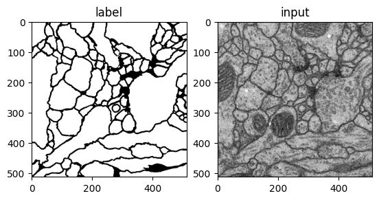
U-Net Modeling
 해당 U-Net의 이미지를 잘 참고하여 U-Net 네트워크를 직접 구현해볼 것이다.
# U-Net Model
class UNet(nn.Module):
def __init__(self):
super(UNet, self).__init__()
# 이미지 상에서 파란색 화살표를 의미
def CBR2d(in_channels, out_channels, kernel_size=3, stride=1, padding=1, bias=True):
layers = []
layers += [nn.Conv2d(in_channels=in_channels, out_channels=out_channels,
kernel_size=kernel_size, stride=stride, padding=padding, bias=bias)]
layers += [nn.BatchNorm2d(num_features=out_channels)] # 배치 정규화 Layer, num_features: 입력 channel의 개수
layers += [nn.ReLU()]
cbr = nn.Sequential(*layers)
return cbr
# Contraction path
self.enc1_1 = CBR2d(in_channels=1, out_channels=64)
self.enc1_2 = CBR2d(in_channels=64, out_channels=64)
self.pool1 = nn.MaxPool2d(kernel_size=2)
self.enc2_1 = CBR2d(in_channels=64, out_channels=128)
self.enc2_2 = CBR2d(in_channels=128, out_channels=128)
self.pool2 = nn.MaxPool2d(kernel_size=2)
self.enc3_1 = CBR2d(in_channels=128, out_channels=256)
self.enc3_2 = CBR2d(in_channels=256, out_channels=256)
self.pool3 = nn.MaxPool2d(kernel_size=2)
self.enc4_1 = CBR2d(in_channels=256, out_channels=512)
self.enc4_2 = CBR2d(in_channels=512, out_channels=512)
self.pool4 = nn.MaxPool2d(kernel_size=2)
self.enc5_1 = CBR2d(in_channels=512, out_channels=1024)
# Expanding path
self.dec5_1 = CBR2d(in_channels=1024, out_channels=512)
self.unpool4 = nn.ConvTranspose2d(in_channels=512, out_channels=512,
kernel_size=2, stride=2, padding=0, bias=True)
self.dec4_2 = CBR2d(in_channels=512*2, out_channels=512) # 동일한 level에서의 Encoder의 출력이 합쳐져야 하므로 in_channels에 2를 곱해준다.
self.dec4_1 = CBR2d(in_channels=512, out_channels=256)
self.unpool3 = nn.ConvTranspose2d(in_channels=256, out_channels=256,
kernel_size=2, stride=2, padding=0, bias=True)
self.dec3_2 = CBR2d(in_channels=256*2, out_channels=256)
self.dec3_1 = CBR2d(in_channels=256, out_channels=128)
self.unpool2 = nn.ConvTranspose2d(in_channels=128, out_channels=128,
kernel_size=2, stride=2, padding=0, bias=True)
self.dec2_2 = CBR2d(in_channels=128*2, out_channels=128)
self.dec2_1 = CBR2d(in_channels=128, out_channels=64)
self.unpool1 = nn.ConvTranspose2d(in_channels=64, out_channels=64,
kernel_size=2, stride=2, padding=0, bias=True)
self.dec1_2 = CBR2d(in_channels=64*2, out_channels=64)
self.dec1_1 = CBR2d(in_channels=64, out_channels=64)
self.fc = nn.Conv2d(in_channels=64, out_channels=1,
kernel_size=1, stride=1, padding=0, bias=True)
def forward(self, x):
enc1_1 = self.enc1_1(x)
enc1_2 = self.enc1_2(enc1_1)
pool1 = self.pool1(enc1_2)
enc2_1 = self.enc2_1(pool1)
enc2_2 = self.enc2_2(enc2_1)
pool2 = self.pool2(enc2_2)
enc3_1 = self.enc3_1(pool2)
enc3_2 = self.enc3_2(enc3_1)
pool3 = self.pool3(enc3_2)
enc4_1 = self.enc4_1(pool3)
enc4_2 = self.enc4_2(enc4_1)
pool4 = self.pool4(enc4_2)
enc5_1 = self.enc5_1(pool4)
dec5_1 = self.dec5_1(enc5_1)
unpool4 = self.unpool4(dec5_1)
# torch.cat을 통해 두 텐서를 dim=1 방향으로 연결한다.
# dim= [0: batch, 1: channel, 2: height, 3: width]
cat4 = torch.cat((unpool4, enc4_2), dim=1)
dec4_2 = self.dec4_2(cat4)
dec4_1 = self.dec4_1(dec4_2)
unpool3 = self.unpool3(dec4_1)
cat3 = torch.cat((unpool3, enc3_2), dim=1)
dec3_2 = self.dec3_2(cat3)
dec3_1 = self.dec3_1(dec3_2)
unpool2 = self.unpool2(dec3_1)
cat2 = torch.cat((unpool2, enc2_2), dim=1)
dec2_2 = self.dec2_2(cat2)
dec2_1 = self.dec2_1(dec2_2)
unpool1 = self.unpool1(dec2_1)
cat1 = torch.cat((unpool1, enc1_2), dim=1)
dec1_2 = self.dec1_2(cat1)
dec1_1 = self.dec1_1(dec1_2)
x = self.fc(dec1_1)
return x 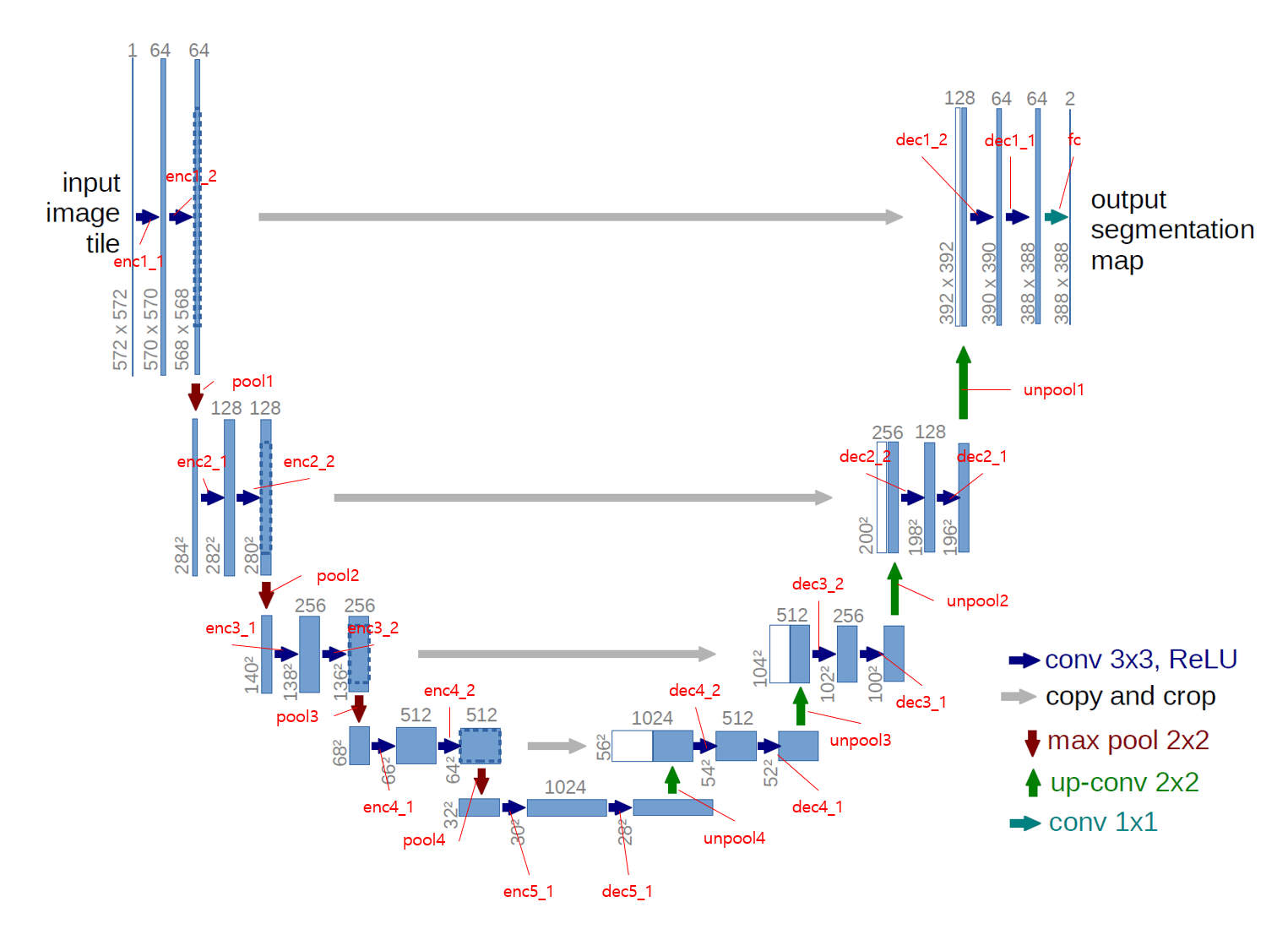 해당 그림을 참고하면 코드를 이해하기 더 편할 것이다.
Dataset Load & Transform
Class를 이용하여 DataLoder와 Transform을 직접 구현해볼 것이다.
## DataLoader 구현

# 데이터셋 경로 재정의
data_dir = './datasets'


class Dataset(torch.utils.data.Dataset):
    def __init__(self, data_dir, transform=None):
        self.data_dir = data_dir
        self.transform = transform

        lst_data = os.listdir(self.data_dir)  # os.listdir를 통해 경로 data_dir에 있는 파일을 불러온다.

        lst_label = [f for f in lst_data if f.startswith('label')]  # lst_data에서 이름이 'label'로 시작하는 파일들을 배열 형태로 저장
        lst_input = [f for f in lst_data if f.startswith('input')]  # lst_data에서 이름이 'input'으로 시작하는 파일들을 배열 형태로 저장

        lst_label.sort()  # 정렬
        lst_input.sort()

        self.lst_label = lst_label
        self.lst_input = lst_input


    def __len__(self):
        return len(self.lst_label)  # length 반환


    def __getitem__(self, index):
        label = np.load(os.path.join(self.data_dir, self.lst_label[index]))  # op.path.join을 통해 해당 index에 맞는 label파일의 경로를 설정 후 load
        input = np.load(os.path.join(self.data_dir, self.lst_input[index]))

        # 0~1로 Normalization
        label = label/255.0
        input = input/255.0

        # Channel이 없다면 임의로 생성해줌
        if label.ndim == 2:
            label = label[:, :, np.newaxis]
        if input.ndim == 2:
            input = input[:, :, np.newaxis]

        data = {'input': input, 'label': label}

        if self.transform:
            data = self.transform(data)

        return data
아래 코드를 통해 index = 0의 Train data의 input과 label을 시각적으로 확인할 수 있다.
dataset_train = Dataset(data_dir=os.path.join(data_dir, 'train'))

data = dataset_train.__getitem__(0)

input = data['input']
label = data['label']


plt.subplot(121)
plt.imshow(input.squeeze())

plt.subplot(122)
plt.imshow(label.squeeze())

plt.show()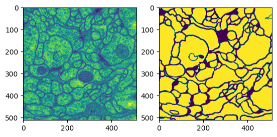
이제 Transform을 구현해줄 것이다.
## Transform 구현

class ToTensor(object):
    def __call__(self, data):
        label, input = data['label'], data['input']


        """
         Image의 numpy 차원 = (Y, X, Ch)이고,
         tensor 차원 = (Ch, Y, X)이므로 이를 바꿔준다.
        """
        label = label.transpose((2, 0, 1)).astype(np.float32)
        input = input.transpose((2, 0, 1)).astype(np.float32)

        data = {'label': torch.from_numpy(label), 'input': torch.from_numpy(input)}

        return data

class Normalization(object):
    def __init__(self, mean=0.5, std=0.5):
        self.mean = mean
        self.std = std

    def __call__(self, data):
        label, input = data['label'], data['input']

        input = (input - self.mean) / self.std

        data = {'label': label, 'input': input}

        return data

class RandomFlip(object):
    def __call__(self, data):
        label, input = data['label'], data['input']

        # 50% 확률로 데이터를 좌우상하 Flip
        if np.random.rand() > 0.5:
            label = np.fliplr(label)
            input = np.fliplr(input)

        if np.random.rand() > 0.5:
            label = np.flipud(label)
            input = np.flipud(input)

        data = {'label': label, 'input': input}

        return data
위 코드에서 볼 수 있는 것 처럼, 데이터셋을 Numpy에서 Tensor로 보내는 기능, Normalization 하는 기능, 50% 확률로 Flip 하는 기능(Data Augmentation)을 구현하였다.
Training
이제 본격적으로 Training을 진행해볼 것이다.
## Training

# Hyper parameter
lr = 1e-3
batch_size = 4
num_epoch = 100

device = torch.device('cuda' if torch.cuda.is_available() else 'cpu')

net = UNet().to(device)

fn_loss = nn.BCEWithLogitsLoss().to(device)  # Loss Function
optim = torch.optim.Adam(net.parameters(), lr=lr)  # Optimizer


transform = transforms.Compose([Normalization(mean=0.5, std=0.5), RandomFlip(), ToTensor()])

# Train 데이터셋, Validation 데이터셋 Load 후 transform
dataset_train = Dataset(data_dir=os.path.join(data_dir, 'train'), transform=transform)
loader_train = DataLoader(dataset=dataset_train, batch_size=batch_size, shuffle=True, num_workers=8)

dataset_val = Dataset(data_dir=os.path.join(data_dir, 'val'), transform=transform)
loader_val = DataLoader(dataset=dataset_val, batch_size=batch_size, shuffle=False, num_workers=8)


# Train, Validation 데이터셋 length 설정
num_data_train = len(dataset_train)
num_data_val = len(dataset_val)

# batch_size에 의해서 나눠지는 Train, Validation set의 수 설정
num_batch_train = np.ceil(num_data_train/batch_size)  # np.ceil을 통해 반올림
num_batch_val = np.ceil(num_data_val/batch_size)
우선 필요한 변수들을 정의한다.
## Network Training Loop

st_epoch = 0  # Start epoch

for epoch in range(st_epoch + 1, num_epoch + 1):
    net.train()
    loss_arr = []

    for batch, data in enumerate(loader_train, 1):
        label = data['label'].to(device)
        input = data['input'].to(device)

        output = net(input)

        optim.zero_grad()

        loss = fn_loss(output, label)
        loss.backward()

        optim.step()

        loss_arr += [loss.item()]

        print("TRAIN: EPOCH %04d / %04d  |  BATCH %04d / %04d  |  LOSS %.4f" %
            (epoch, num_epoch, batch, num_batch_train, np.mean(loss_arr)))


    ## Network Validation Loop
    with torch.no_grad():
        net.eval()
        loss_arr = []

        for batch, data in enumerate(loader_val, 1):
            label = data['label'].to(device)
            input= data['input'].to(device)

            output = net(input)

            loss = fn_loss(output, label)
            loss_arr += [loss.item()]

            print("VALID: EPOCH %04d / %04d  |  BATCH %04d / %04d  |  LOSS %.04f" %
                (epoch, num_epoch, batch, num_batch_val, np.mean(loss_arr)))

torch.save(net.state_dict(), './model.pth')TRAIN: EPOCH 0001 / 0100 | BATCH 0001 / 0006 | LOSS 0.7724
TRAIN: EPOCH 0001 / 0100 | BATCH 0002 / 0006 | LOSS 0.7059
TRAIN: EPOCH 0001 / 0100 | BATCH 0003 / 0006 | LOSS 0.6668
TRAIN: EPOCH 0001 / 0100 | BATCH 0004 / 0006 | LOSS 0.6431
TRAIN: EPOCH 0001 / 0100 | BATCH 0005 / 0006 | LOSS 0.6157
TRAIN: EPOCH 0001 / 0100 | BATCH 0006 / 0006 | LOSS 0.5951
VALID: EPOCH 0001 / 0100 | BATCH 0001 / 0001 | LOSS 0.6519
TRAIN: EPOCH 0002 / 0100 | BATCH 0001 / 0006 | LOSS 0.4961
TRAIN: EPOCH 0002 / 0100 | BATCH 0002 / 0006 | LOSS 0.4712
TRAIN: EPOCH 0002 / 0100 | BATCH 0003 / 0006 | LOSS 0.4607
TRAIN: EPOCH 0002 / 0100 | BATCH 0004 / 0006 | LOSS 0.4495
TRAIN: EPOCH 0002 / 0100 | BATCH 0005 / 0006 | LOSS 0.4432
TRAIN: EPOCH 0002 / 0100 | BATCH 0006 / 0006 | LOSS 0.4366
VALID: EPOCH 0002 / 0100 | BATCH 0001 / 0001 | LOSS 0.5309
TRAIN: EPOCH 0003 / 0100 | BATCH 0001 / 0006 | LOSS 0.3950
TRAIN: EPOCH 0003 / 0100 | BATCH 0002 / 0006 | LOSS 0.3969
TRAIN: EPOCH 0003 / 0100 | BATCH 0003 / 0006 | LOSS 0.3931
TRAIN: EPOCH 0003 / 0100 | BATCH 0004 / 0006 | LOSS 0.3921
TRAIN: EPOCH 0003 / 0100 | BATCH 0005 / 0006 | LOSS 0.3874
TRAIN: EPOCH 0003 / 0100 | BATCH 0006 / 0006 | LOSS 0.3836
VALID: EPOCH 0003 / 0100 | BATCH 0001 / 0001 | LOSS 0.5030
TRAIN: EPOCH 0004 / 0100 | BATCH 0001 / 0006 | LOSS 0.3593
TRAIN: EPOCH 0004 / 0100 | BATCH 0002 / 0006 | LOSS 0.3550
TRAIN: EPOCH 0004 / 0100 | BATCH 0003 / 0006 | LOSS 0.3498
TRAIN: EPOCH 0004 / 0100 | BATCH 0004 / 0006 | LOSS 0.3517
...
TRAIN: EPOCH 0100 / 0100 | BATCH 0004 / 0006 | LOSS 0.1543
TRAIN: EPOCH 0100 / 0100 | BATCH 0005 / 0006 | LOSS 0.1558
TRAIN: EPOCH 0100 / 0100 | BATCH 0006 / 0006 | LOSS 0.1581
VALID: EPOCH 0100 / 0100 | BATCH 0001 / 0001 | LOSS 0.2070
Training Loop와 Validation Loop를 구성해준다. 모든 Loop가 끝난 후에는 모델을 저장해준다.
Test
Model의 Training을 마친 후에 Test를 진행할 것이다.
results 폴더를 만든 후 Test의 결과를 numpy와 png 형태로 저장할 것이다.
## Test

transform = transforms.Compose([Normalization(mean=0.5, std=0.5), ToTensor()])

# Test 데이터셋 Load 후 transform
dataset_test = Dataset(data_dir=os.path.join(data_dir, 'test'), transform=transform)
loader_test = DataLoader(dataset=dataset_test, batch_size=batch_size, shuffle=False, num_workers=8)


# Test 데이터셋 length 설정
num_data_test = len(dataset_test)


# batch_size에 의해서 나눠지는 Test set의 수 설정
num_batch_test = np.ceil(num_data_test/batch_size)  # np.ceil을 통해 반올림


# Output을 저장하기 위한 functions
fn_tonumpy = lambda x: x.to('cpu').detach().numpy().transpose(0, 2, 3, 1)  # tensor to numpy
fn_denorm = lambda x, mean, std: (x * std) + mean  # Normalization 되어있는 데이터를 Denormalization
fn_class = lambda x: 1.0 * (x > 0.5)  # Network output의 이미지를 binary class로 분류
Test에 필요한 변수와 함수들을 구현한다.
result_dir = './results'

if not os.path.exists(result_dir):
    os.makedirs(result_dir)
    os.makedirs(os.path.join(result_dir, 'png'))
    os.makedirs(os.path.join(result_dir, 'numpy'))
프로젝트 폴더 내에 results 폴더를 만들어 준 후, png 파일과 numpy 파일을 저장할 하위 폴더들을 만들어준다.
이제 Test를 위한 Loop를 구현해줄 것이다.
## Network Test Loop

st_epoch = 0

with torch.no_grad():
    net.eval()
    loss_arr = []

    for batch, data in enumerate(loader_test, 1):
        label = data['label'].to(device)
        input= data['input'].to(device)

        output = net(input)

        loss = fn_loss(output, label)
        loss_arr += [loss.item()]

        print("TEST:BATCH %04d / %04d  |  LOSS %.4f" %
            (batch, num_batch_test, np.mean(loss_arr)))

        label = fn_tonumpy(label)
        input = fn_tonumpy(fn_denorm(input, mean=0.5, std=0.5))
        output = fn_tonumpy(fn_class(output))

        for j in range(label.shape[0]):
            id = num_batch_test * (batch -1) + j

            plt.imsave(os.path.join(result_dir, 'png', 'label_%04d.png' % id), label[j].squeeze(), cmap='gray')
            plt.imsave(os.path.join(result_dir, 'png', 'input_%04d.png' % id), input[j].squeeze(), cmap='gray')
            plt.imsave(os.path.join(result_dir, 'png', 'output_%04d.png' % id), output[j].squeeze(), cmap='gray')

            np.save(os.path.join(result_dir, 'numpy', 'label_%04d.npy' % id), label[j].squeeze())
            np.save(os.path.join(result_dir, 'numpy', 'input_%04d.npy' % id), input[j].squeeze())
np.save(os.path.join(result_dir, 'numpy', 'output_%04d.npy' % id), output[j].squeeze())TEST:BATCH 0001 / 0001 | LOSS 0.1718Test가 끝났다면 results 폴더 내 png 폴더에서 input, label, output을 시각적으로 확인할 수 있다.
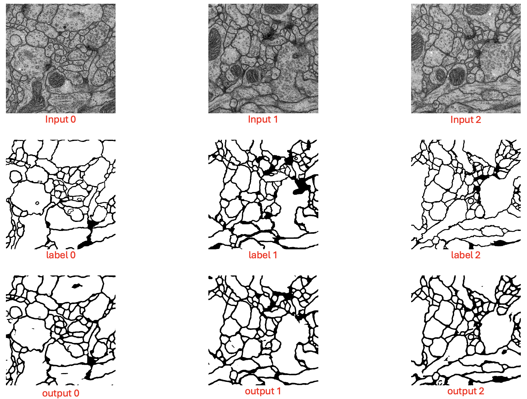 label과 output이 매우 정교하게 일치하는 건 아니지만 괜찮은 성능으로 Segmentation 하는 것을 확인할 수 있다.