코딩테스트 연습
알고리즘
def solution(dartResult):
    squared = {
        'S':1
        , 'D':2
        , 'T':3
    }
    temp = ''
    score = []
    for i in dartResult:
        if i.isdigit():
            temp += i
        elif i.isalpha():
            score.append(pow(int(temp), squared[i]))
            temp = ''
        elif i == '*':
            if len(score) > 1:
                score[-2] *= 2
            score[-1]*=2
        elif i == '#':
            score[-1] *= -1
return sum(score)import re
def solution(dartResult):
# 1. 정규식을 사용하여 점수와 보너스, 옵션을 추출
rounds = re.findall(r'(\d+)([SDT])([*#]?)', dartResult)
scores = [] # 점수를 저장할 리스트
for i, (score, bonus, option) in enumerate(rounds):
# 2. 점수 변환 및 보너스 처리
score = int(score)
if bonus == 'S':
score **= 1
elif bonus == 'D':
score **= 2
elif bonus == 'T':
score **= 3
# 3. 옵션 처리
if option == '*':
score *= 2
if i > 0: # 이전 점수도 2배
scores[i - 1] *= 2
elif option == '#':
score *= -1
# 점수를 리스트에 저장
scores.append(score)
# 총점 반환
return sum(scores)- 정규식을 사용해 문자열 파싱
\d+: 숫자(점수) 추출[SDT]: 보너스 구분 추출[*#]?: 옵션 추출 (없을 수도 있음)
1D#2S*3S를 넣으면:
[('1', 'D', '#'), ('2', 'S', '*'), ('3', 'S', '')] 생성
1D2S3T*를 넣으면:
[('1', 'D', ''), ('2', 'S', ''), ('3', 'T', '*')]- 점수와 보너스 계산
- 옵션 처리
- 스타상(
*)- 현재 점수와 이전 점수를 2배로 만듦
- 첫 번째 기회에서도 나올 수 있음 → 이 경우 첫 번째 스타상(
*)의 점수만 2배 - 중복 적용 가능
- 아차상과도 중복 가능
- 아차상(
#)- 현재 점수에 -1을 곱함
- 스타상과 중복 가능 → 이 경우 중첩된 아차상(#)의 점수는 -2배
- 스타상(
- 점수 계산 부분을 따로 함수로 빼도 됨
import re

def SDT(num, c):
    if c == 'S' : return num
    elif c == 'D' : return num ** 2
    else : return num ** 3

def solution(dartResult):
    answer = []
    dart = re.findall(r'\d+|[a-zA-Z][^\d\s]*',dartResult) 	# 숫자 또는 문자+특수문자 조합 찾음

    for idx, chars in zip(range(1,len(dart)+1,2),dart[1::2]):
        answer.append(SDT(int(dart[idx-1]),chars[0])) 	# 숫자,(Single/Double/Triple 연산)

        if len(chars) == 2 :
            if chars[1] == '*':
                answer[len(answer)-1] *= 2
                if len(answer) != 1 : answer[len(answer)-2] *= 2
            elif chars[1] == '#':
                answer[len(answer)-1] *= (-1)

return sum(answer)- compile 활용
import re

def solution(dartResult):
    bonus = {'S' : 1, 'D' : 2, 'T' : 3}
    option = {'' : 1, '*' : 2, '#' : -1}
    p = re.compile('(\d+)([SDT])([*#]?)')
    dart = p.findall(dartResult)

    for i in range(len(dart)):
        if dart[i][2] == '*' and i > 0:
            dart[i-1] *= 2
        dart[i] = int(dart[i][0]) ** bonus[dart[i][1]] * option[dart[i][2]]
    answer = sum(dart)
return answer- 또다른 풀이
def solution(dartResult):
    shots = ['']  # shots[i] = i회차의 결과(str). shots[0] = ''
    points = [0]  # points[i] = i회차로 얻은 점수(int). points[0] = 0
    muls = {'S':1,'D':2,'T':3}  # (i영역 점수) **= muls[i]

    s, p = '', ''  # 각각 dartResult의 결과 부분, 점수 부분 (str)
    strs = {'S','D','T','*','#'}  # 결과 부분을 이루는 문자들

    split = False  # 회차가 구분되는 지점인지의 여부.

    for i in dartResult:
        if i.isdigit():
            if split:  # 만약 회차가 구분되는 지점이라면
                shots.append(s)  # shots에 결과 부분(str) 저장
                points.append(int(p))  # point에 점수 부분(int) 저장
                s, p = '', ''  # 이후 결과 부분, 점수 부분과
                split = False  # '회차가 구분되는 지점인지' 여부를 초기화한다
            p += i
        else:
            s += i
            split = True
    shots.append(s)  # 리스트: shots 완성
    points.append(int(p))  # 리스트: points 완성

    for i in range(1,4):  # 1 ~ 3회차 점수 계산
        points[i] **= muls[shots[i][0]]
        if len(shots[i]) == 2:
            if shots[i][1] == '*':  # 스타상 효과 적용
                points[i-1] *= 2
                points[i] *= 2
            elif shots[i][1] == '#':  # 아차상 효과 적용
                points[i] *= -1

    return sum(points)
SQL
SELECT
    id
    , SUM(IF(month="Jan", revenue, null)) AS Jan_Revenue
    , SUM(IF(month="Feb", revenue, null)) AS Feb_Revenue
    , SUM(IF(month="Mar", revenue, null)) AS Mar_Revenue
    , SUM(IF(month="Apr", revenue, null)) AS Apr_Revenue
    , SUM(IF(month="May", revenue, null)) AS May_Revenue
    , SUM(IF(month="Jun", revenue, null)) AS Jun_Revenue
    , SUM(IF(month="Jul", revenue, null)) AS Jul_Revenue
    , SUM(IF(month="Aug", revenue, null)) AS Aug_Revenue
    , SUM(IF(month="Sep", revenue, null)) AS Sep_Revenue
    , SUM(IF(month="Oct", revenue, null)) AS Oct_Revenue
    , SUM(IF(month="Nov", revenue, null)) AS Nov_Revenue
    , SUM(IF(month="Dec", revenue, null)) AS Dec_Revenue
FROM
    Department
GROUP BY
    id
;- CASE WHEN 사용
select id,
sum(case when month = "Jan" then revenue else NULL end) as Jan_Revenue,
sum(case when month = "Feb" then revenue else NULL end) as Feb_Revenue,
sum(case when month = "Mar" then revenue else NULL end) as Mar_Revenue,
sum(case when month = "Apr" then revenue else NULL end) as Apr_Revenue,
sum(case when month = "May" then revenue else NULL end) as May_Revenue,
sum(case when month = "Jun" then revenue else NULL end) as Jun_Revenue,
sum(case when month = "Jul" then revenue else NULL end) as Jul_Revenue,
sum(case when month = "Aug" then revenue else NULL end) as Aug_Revenue,
sum(case when month = "Sep" then revenue else NULL end) as Sep_Revenue,
sum(case when month = "Oct" then revenue else NULL end) as Oct_Revenue,
sum(case when month = "Nov" then revenue else NULL end) as Nov_Revenue,
sum(case when month = "Dec" then revenue else NULL end) as Dec_Revenue
from Department
group by id
order by id
;- WINDOW FUNCTION SUM OVER () 사용
SELECT
    DISTINCT id
    , SUM(CASE WHEN month = "Jan" THEN revenue END) OVER (PARTITION BY id ORDER BY (SELECT NULL)) AS Jan_Revenue
    , SUM(CASE WHEN month = "Feb" THEN revenue END) OVER (PARTITION BY id ORDER BY (SELECT NULL)) AS Feb_Revenue
    , SUM(CASE WHEN month = "Mar" THEN revenue END) OVER (PARTITION BY id ORDER BY (SELECT NULL)) AS Mar_Revenue
    , SUM(CASE WHEN month = "Apr" THEN revenue END) OVER (PARTITION BY id ORDER BY (SELECT NULL)) AS Apr_Revenue
    , SUM(CASE WHEN month = "May" THEN revenue END) OVER (PARTITION BY id ORDER BY (SELECT NULL)) AS May_Revenue
    , SUM(CASE WHEN month = "Jun" THEN revenue END) OVER (PARTITION BY id ORDER BY (SELECT NULL)) AS Jun_Revenue
    , SUM(CASE WHEN month = "Jul" THEN revenue END) OVER (PARTITION BY id ORDER BY (SELECT NULL)) AS Jul_Revenue
    , SUM(CASE WHEN month = "Aug" THEN revenue END) OVER (PARTITION BY id ORDER BY (SELECT NULL)) AS Aug_Revenue
    , SUM(CASE WHEN month = "Sep" THEN revenue END) OVER (PARTITION BY id ORDER BY (SELECT NULL)) AS Sep_Revenue
    , SUM(CASE WHEN month = "Oct" THEN revenue END) OVER (PARTITION BY id ORDER BY (SELECT NULL)) AS Oct_Revenue
    , SUM(CASE WHEN month = "Nov" THEN revenue END) OVER (PARTITION BY id ORDER BY (SELECT NULL)) AS Nov_Revenue
    , SUM(CASE WHEN month = "Dec" THEN revenue END) OVER (PARTITION BY id ORDER BY (SELECT NULL)) AS Dec_Revenue
FROM
    Department
;
지난 시간 복습
- 선형 회귀 모델링:
linear_model = LinearRegression()
- 선형 모델의 원리: 데이터를 잘 대표하는 직선을 찾아나가는 과정
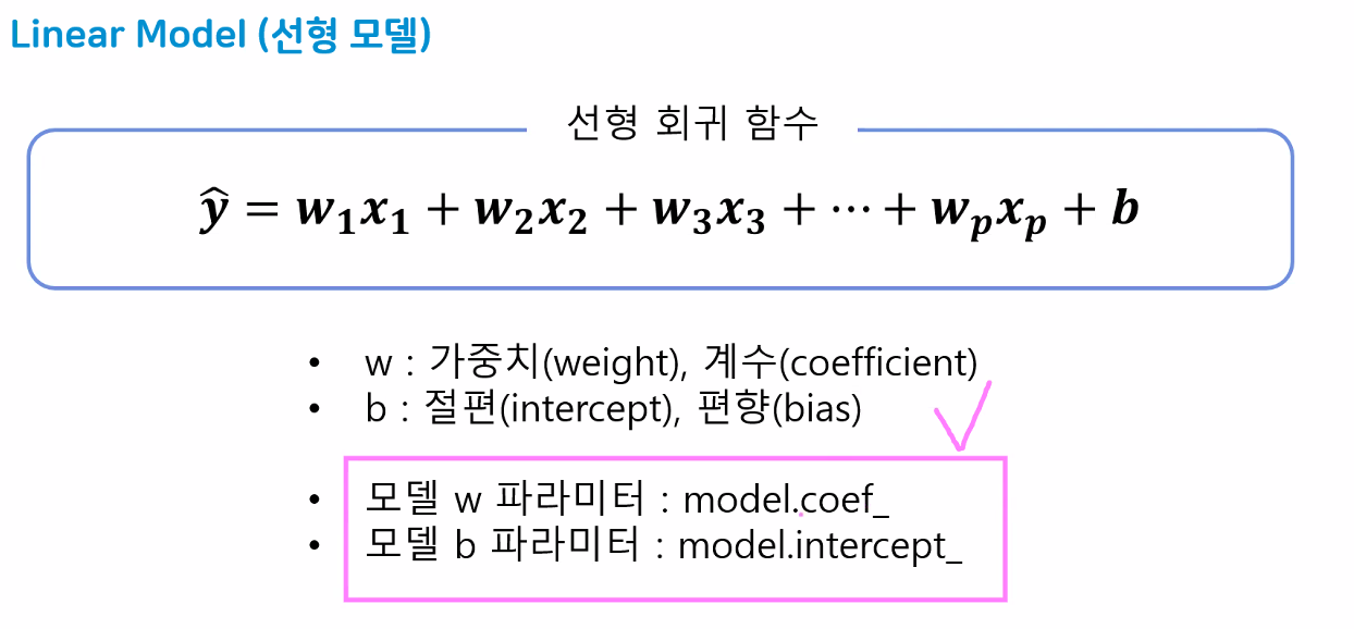
- w의 개수만큼 가중치가 나옴
- 43개의 입력 특성 → 43개의 가중치
- 가중치 순서는 컬럼 순서(data.columns)와 동일
- 선형 모델의 원리: 데이터를 잘 대표하는 직선을 찾아나가는 과정
- 모델 평가: 선형 회귀 모델의 score는 뭘까?
- 분류 모델의 경우 model.score는 accuracy(정확도)
- 전체 데이터 중에서 O/X → 맞춘 데이터 비율
- 회귀 모델은 오차 기반의 평가 지표 도구 사용(오차 정도를 평가 지표로 활용)
- MSE(mean square error; 평균 제곱 오차)
- 분류 모델의 경우 model.score는 accuracy(정확도)
- MSE(mean_square_error)
- 사이킷런 평가지표 모음집인 .metrics 안에 있음
- 실제값(y)과 예측값()의 차이(=오차 정도)
- 오차가 크면 많이 수정 → 오차를 극대화시켜 수정하기 쉽게 하려고 제곱
- 평균 "제곱" 오차이기 때문에 단위도 제곱됨 → 루트를 씌워 해결:
RMSE- 또 다른 해결법: 절댓값을 사용한 지표→
MAE
- 또 다른 해결법: 절댓값을 사용한 지표→
- 모델 평가 지표
- 분류: accuracy(정확도) 지표를 대표적으로 사용
- 정답 데이터가 범주형 -> 전체 데이터에서 맞은 데이터의 개수를 확률로 표현
- 0 ~ 1 사이의 숫자로 출력
- 1에 가까울수록 좋은 모델
- 회귀: 오차 기반의 평가지표를 사용한다.
- 오차가 크니? 작니?에 따라서 모델의 성능을 평가한다!
- mse(평균제곱오차, mean_squared_error)
- mse 지표는 학습과 평가 모두 사용된다!
- 분류: accuracy(정확도) 지표를 대표적으로 사용
- 선형 회귀 모델의 평가 지표
- MSE: 평균제곱오차(
mean_squared_error)- 지표가 작을수록 잘 예측하는 모델(
오차 기반 평가 지표)
- 지표가 작을수록 잘 예측하는 모델(
- RMSE: mse에 루트를 씌운 값
- 해석 시 단위 문제를 해결하기 위해 mse에 루트를 씌워 수치를 정상화
- MAE: 평균 절댓값 오차(
mean_absolute_error)- 오차를 절댓값으로 변환하여 평균을 구한 값
- MSE에 비해 오차에 덜 민감
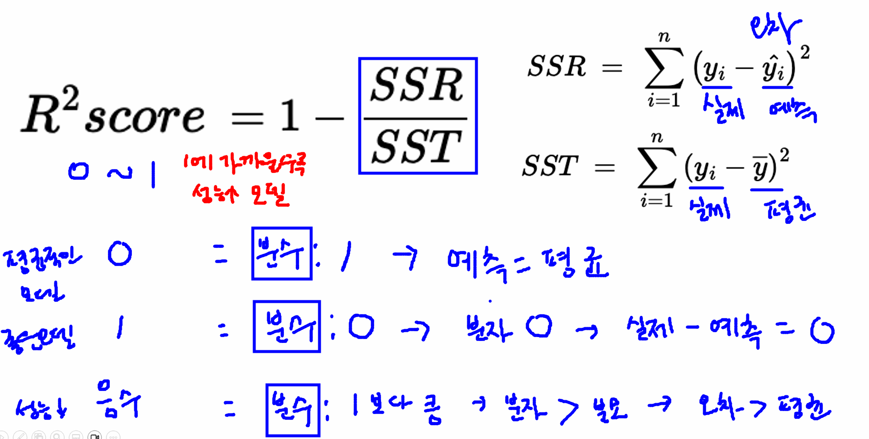
- score: 오차와 평균값을 활용하여 정규화된 평가가 가능하도록 만든 평가 지표
- 0~1 사이의 값을 주로 가지며
- 0에 가까울수록 평균적인 성능을 가지는 모델 (좋은 편X)
- 1에 가까울수록 좋은 성능을 가지는 모델
- 음수: 성능이 매우 좋지 않은 모델
- MSE: 평균제곱오차(
- 회귀 모델은 오차 기반 평가 진행 BUT 오차는 판단하기 어려움: "그래서 오차가 큰 거야? 작은 거야?"
- 오차 기반은 평가가 애매함 → 3억 차이라고 하면:
- 집값이 100억인데 3억 차이면 예측 잘 한 것
- 집값이 10억인데 3억 차이면 예측 잘 못한 것
- 즉, 정규화된 평가 지표가 필요!
- 해당 데이터 분야의 전문가가 아니라면 확인이 힘듦
- 오차는 판단하는 사람마다 다르게 느낄 수 있기 때문에 정규화된 방법으로 평가가 필요 → score로 해결
- 오차 기반은 평가가 애매함 → 3억 차이라고 하면:
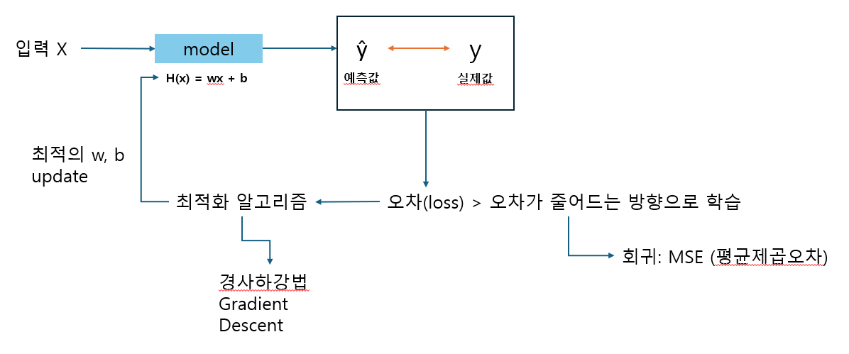
- 경사하강법(Gradient Descent)
- 손실함수(loss function)의 값을 최소화 == 오차를 최소화
- 이를 위해 가중치(w), 절편(b_)을 반복적으로 업데이트
- 손실함수의 기울기(→미분) 따라 가장 빠르게 감소하는 방향으로 파라미터를 이동시켜 최솟값에 도달
- 기울기가 최소가 되는 지점의 w값을 예측해 나가는 과정
- 가중치와 절편의 초기값은 랜덥 → 설정된 초기값에서 다음 발자국으로 '이동' → 이동할 때 보폭의 크기 == learning rate
- 학습률(learning rate) == 보폭
- 하이퍼파라미터 중 하나
- 기본값은 보통 0.1 or 0.01
- 학습률이 너무 크면 발산 → 비효율
- 학습률이 너무 그면 수렴 속도가 너무 느림 → 최솟값 도착 전 정해진 학습 횟수(epochs) 종료될 위험성
- 손실함수(loss function)의 값을 최소화 == 오차를 최소화
- X: 특성이 1개여도 반드시 2차원으로 만들어야 함!
- 입력 받는 데이터를 2차원으로 주는 것이 머신러닝의 default
- 우리가 앞서 사용한 LinearRegression 모델은 정규계산식을 사용함(경사하강법 아님)
- 따라서 경사하강법을 사용하는 모델을 추가로 다룰 것 → SGD(Stochastic Gradient Descent): 경사하강법을 사용하는 모델(이름에 이미 GD(gradient descent)가 들어있다.)
경사하강법 그래프
# 가설함수 h(x)
def h(w, x):
    return w*x + 0

# 비용함수, 손실함수 (mse)
def loss (data, target, weight):
    # 예측할 데이터의 X: data, 실제 답: target, 예측가중치: weight
    y_pre = h(weight, data)
    mse = np.mean((target - y_pre)**2)
    return mse

# 예측한 가중치가 10
loss(score["시간"], score["성적"], 10) # np.float64(0.0)

# 예측한 가중치가 5
loss(score["시간"], score["성적"], 5) # np.float64(1031.25)

# 예측한 가중치가 15
loss(score["시간"], score["성적"], 15) # np.float64(1031.25)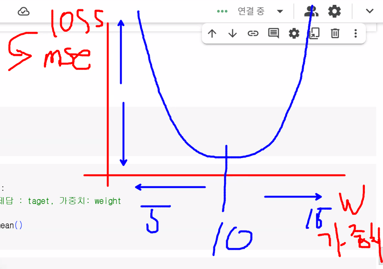
- 가중치 변화에 따른 loss 변화 그래프
- mse를 통해 손실함수(loss)를 확인
- 가설함수 h(x) 생성 이유: 예측값(y_pre) 구하기 위해
- w값이 변함에 따라 y_pred가 달라저야 하는데 모델을 쓰면 값이 하나만 나옴
# x축의 범위 (예측가중치의 변화) -> -10~30
w_arr = range(-10, 30+1)

# mse를 리스트에 저장 (반복)
loss_list = []
for w in w_arr:
    mse = loss(score["시간"], score["성적"], w)
loss_list.append(mse)- append 대신 리스트 컴프리헨션 써도 됨
# 간단한 반복문 -> 리스트 안에 누적할 때 사용
# 리스트명 = [반복하여 담을 데이터 for i in range()]
loss_list = [loss(score["시간"], score["성적"], w) for w in w_arr]- matplotlib plot 그래프
plt.subplots()
plt.plot(w_arr, loss_list) # x축, y축
plt.xlabel("w")
plt.ylabel("loss")
# 그래프를 보는 사람이 이해할 수 있도록 label 적는 습관 가지기
plt.show()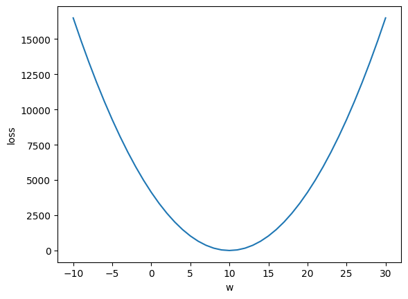
SGDRegressor 모델
- 경사하강법을 활용한 모델
- Stochastic Gradient Descent(확률적 경사하강법)
- 사이킷런에서 제공하는 경사하강법을 활용한 선형 회귀 모델
- 경사하강법을 이용하여 w, b값을 업데이트
- 하이퍼파라미터
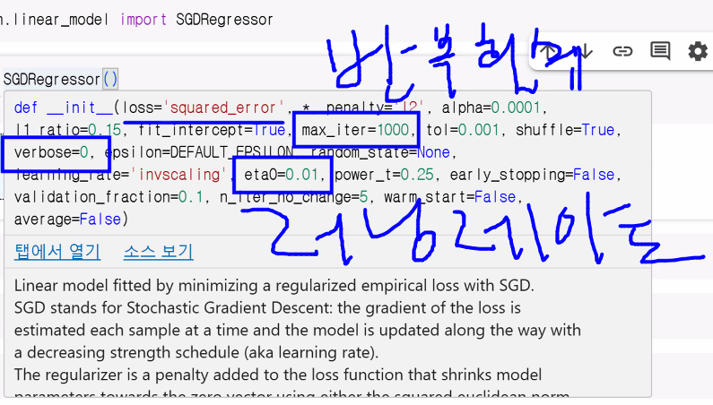
- max_iter: 반복 횟수 설정
- eta0: learning_rate(학습률)
- verbose: 학습 과정(업데이트 과정) 출력 여부
- 0: 출력 안 함
- 1: 출력함
from sklearn.linear_model import SGDRegressor

sgd_model = SGDRegressor()
sgd_model.fit(score[["시간"]], score["성적"])- Q. 강사님과 가중치, 절편이 달라요!
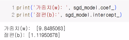
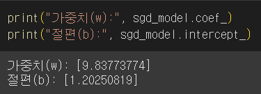
- A. 초기 선택값(가중치와 절편)이 랜덤이기 때문에 동일한 값이 나올 수는 없음
- 그래도 최적의 값으로 잘 찾아갑니다!
- A. 초기 선택값(가중치와 절편)이 랜덤이기 때문에 동일한 값이 나올 수는 없음
print("가중치(w):", sgd_model.coef_)
print("절편(b):", sgd_model.intercept_)

# R2 score 확인하기
sgd_model.score(X = score[["시간"]], y = score["성적"])

# 1에 가까울수록 성능이 좋은 모델~
하이퍼파라미터 조절
sgd_model2 = SGDRegressor(
    eta0 = 0.0001, # 러닝레이트: 기본값 0.01
    max_iter = 5000, # w, b값 업데이트 횟수, 기본값 1000
    verbose = 1 # 학습진행상황 출력 -> 학습 업데이트마다의 결과값 확인
)
sgd_model2.fit(score[["시간"]], score["성적"])

# Epoch: 학습 반복 횟수

sgd_model2.score(score[["시간"]], score["성적"])- 확인해야 하는 것:
- 어떤 하이퍼파라미터를 사용해 성능을 높일 것인가?
집값 데이터를 SGD 모델로 학습 및 평가 진행
sgd_model_tuning = SGDRegressor(
    eta0 = 0.0001,
    max_iter = 10000,
    verbose=1
)
sgd_model_tuning.fit(X = X_train, y = y_train)
sgd_model_tuning.score(X_test, y_test)- score가 0.5 정도인 모델을 믿고 투자할 수 있을까? 성능을 더 높이려면 어떻게 해야 할까?
- 점수를 높일 수 있는 가장 빠른 방법 → 데이터 스케일링!
거리 계산을 하는 모델은 데이터의 스케일이 중요합니다!
데이터 스케일링을 통한 성능 올리기
- 학습의 안정성을 위해 데이터 스케일링을 사용
- StandardScaler 사용
- 선형 모델은 데이터 스케일링을 꼭 해주는 걸 추천
# 강사님 코드
from sklearn.preprocessing import StandardScaler

# 스케일러 객체 생성
st_scaler = StandardScaler()

# 우리의 데이터에 맞게 학습 후 데이터를 반환
X_train_scaled = st_scaler.fit_transform(X_train)
# test 데이터도 변환
# 주의! test 데이터는 변환만! (학습 X)
X_test_scaled = st_scaler.transform(X_test)

# 모델 생성 및 학습
sgd_model4 = SGDRegressor(eta0=0.0001)
sgd_model4.fit(X_train_scaled, y_train)
sgd_model4.score(X_test_scaled, y_test)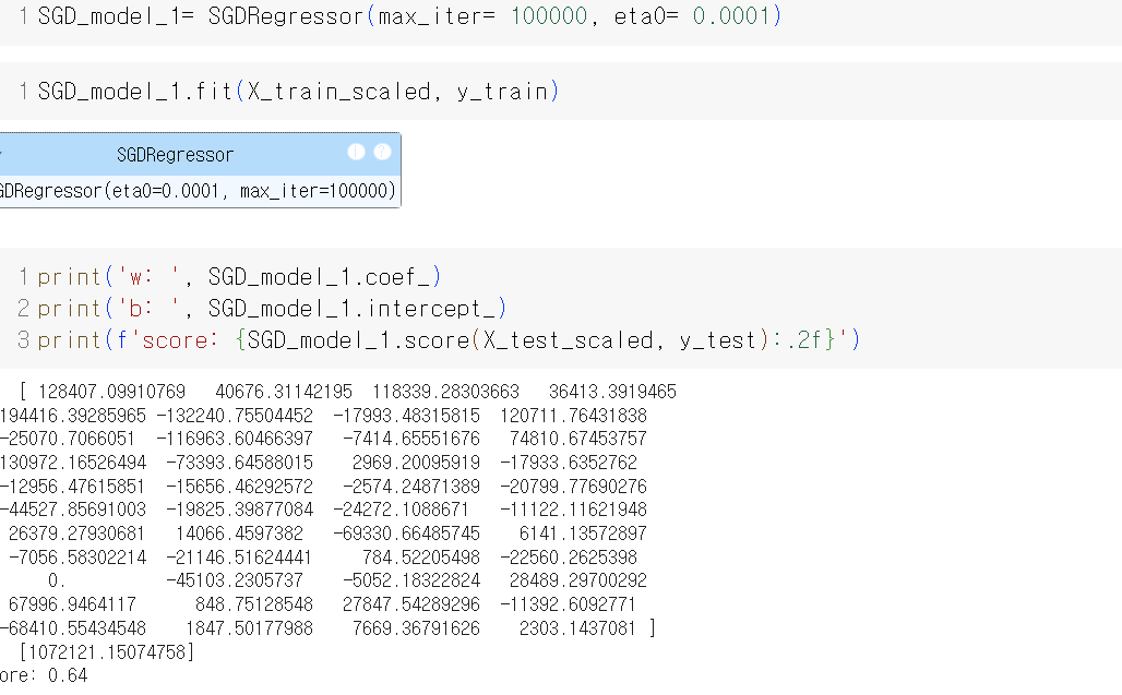
선형 분류 모델
학습 목표
- 선형 분류모델을 이해하고 사용할 수 있다.
- 다양한 분류 평가 지표를 이해할 수 있다.
분류용 선형 모델
- Linear Model (Classification)
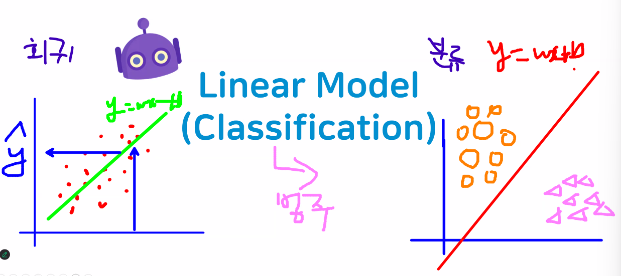
- 회귀: 데이터를 가장 잘 대표하는 직선 그리기
- 분류: 데이터를 가장 잘 나누는 직선 그리기
- 선형모델 → 직선을 그려 나가는 것은 동일
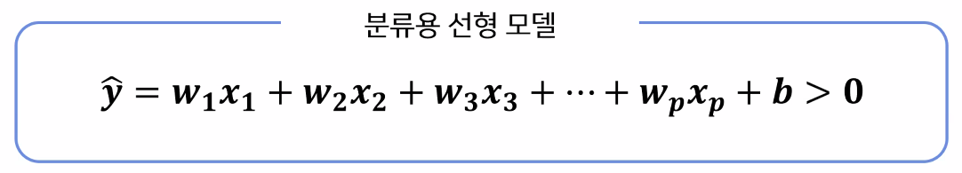
- 분류형 선형 모델은 "결정 경계"가 입력의 선형함수
- 경계선 역할 (대표 X)
- 특성들의 가중치 합이 0보다 크면 class를 +1(양성 클래스)로 분류
- 특성들의 가중치 합이 0보다 작다면 class를 -1(음성 클래스)로 분류
- 경계선 역할 (대표 X)
- 분류 모델
- Logistic Regression(로지스틱 회귀모델)
- 이름에 속지 마시오: "분류용 모델"임
- 회귀에 기반을 두고 있어(원리를 회귀 모델에서 따왔음 -> 선형 회귀와 동일하게 선형 방정식을 학습함) Regression 단어가 붙지만 분류를 더 잘해서 분류 모델로 사용하고 있다고 함
- Linear Support Vector Mashine(SVM)
- Logistic Regression(로지스틱 회귀모델)
로지스틱 회귀모델
- 일반 모델을 사용했을 때 문제점
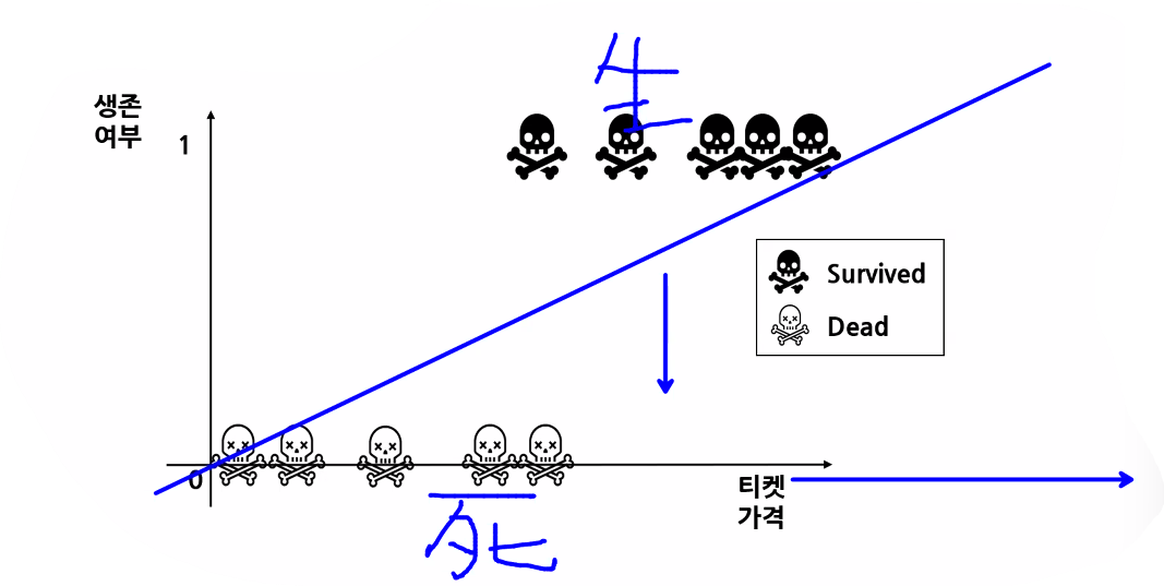
- 일반 모델(단순 직선 모델)은 발산하기 때문에 실제 티켓 가격이 높은 사람은 1등급 손님이고 객실도 높은 층(A)이라서 살 확률이 더 높은데도 죽었다고 분류할 가능성이 있음
- 직선은 양 극단이 발산하기 때문에 분류를 제대로 예측하기 어려움
- 중간에 있는 값(가운데 값)을 얼마나 잘 나누는지가 가장 중요함
- 공부 시간에 따른 합격 여부 → 특정 시간 이상 공부한 사람들은 대부분 합격하지만 중간인 사람은 합격할 수도, 불합격할 수도 있기 때문
- 일반 모델(단순 직선 모델)은 발산하기 때문에 실제 티켓 가격이 높은 사람은 1등급 손님이고 객실도 높은 층(A)이라서 살 확률이 더 높은데도 죽었다고 분류할 가능성이 있음
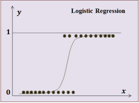
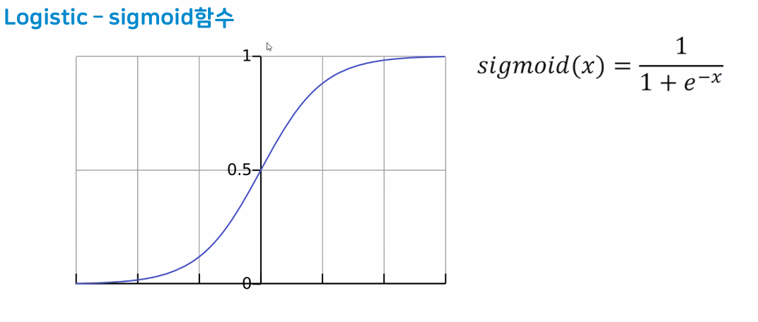
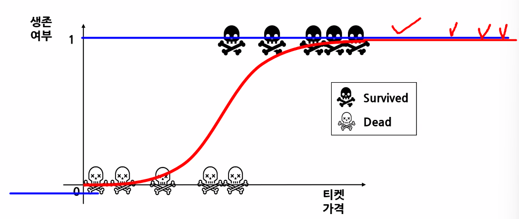
- 시그모이드 함수를 활용해 데이터를 분류
- 0.5를 기준으로 위/아래 분류!
- 시그모이드 함수(또는 로지스틱 함수) 특징
- z가 무한하게 큰 음수일 경우 0에 가까워지고, 무한하게 큰 양수가 될 땐 1에 가까워진다. (가까워지기만 할 뿐 수렴하지는 않음)
- z=0일 땐 0.5가 된다.
- z가 어떤 값이 되더라도 시그모이드 함수는 절대 0~1 사이의 범위를 벗어날 수 없어 해당 값을 0~100% 값으로 해석할 수 있음
- 시그모이드 함수의 출력이 0.5보다 크면 양성 클래스, 작으면 음성 클래스로 판단
- 0.5의 경우 라이브러리마다 판단 다름(사이킷런은 음성 클래스로 판단)
- 0.5를 기준으로 위/아래 분류!
- 분류는 오차와 달리 mse를 사용하지 않음
- 오차가 크면 수정도 많이 해 줘야 하는데 분류는 0/1이라 분류에서 오차 공식으로 mse를 사용하면 상대적으로 작게 나와 수정을 많이 해 줄 수 없음 (1은 제곱해도 1이니까)
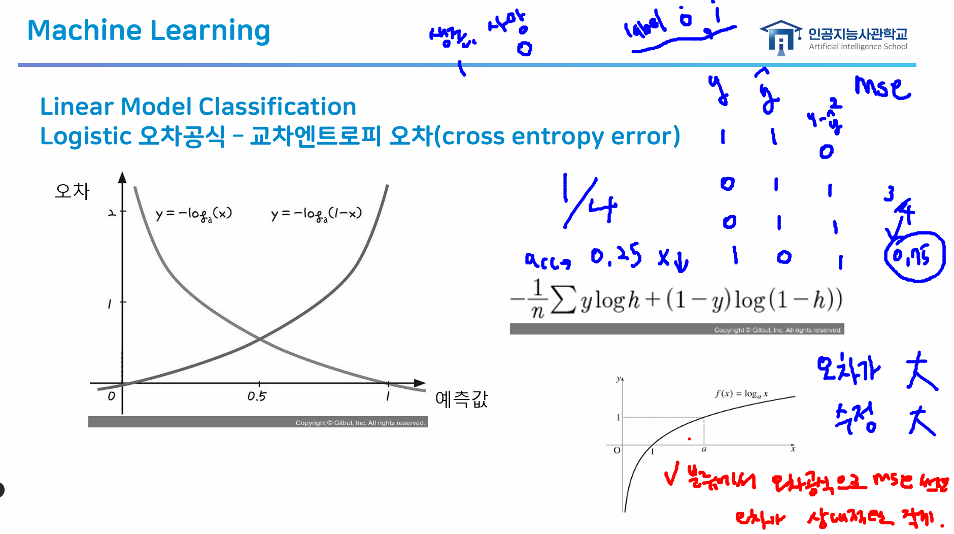
- 따라서 분류에서는 "교차엔트로피 오차"를 사용!
- 오차가 크면 수정도 많이 해 줘야 하는데 분류는 0/1이라 분류에서 오차 공식으로 mse를 사용하면 상대적으로 작게 나와 수정을 많이 해 줄 수 없음 (1은 제곱해도 1이니까)
교차엔트로피 오차(cross entropy error) ★
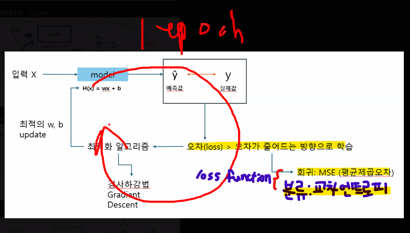
→ 1 epoch 과정마다 오차를 확인해 오차가 줄어드는 방향으로 학습하는 것이 전체적인 모델의 원리
- 교차엔트로피 오차는 로그 함수를 사용해 오차를 극대화함
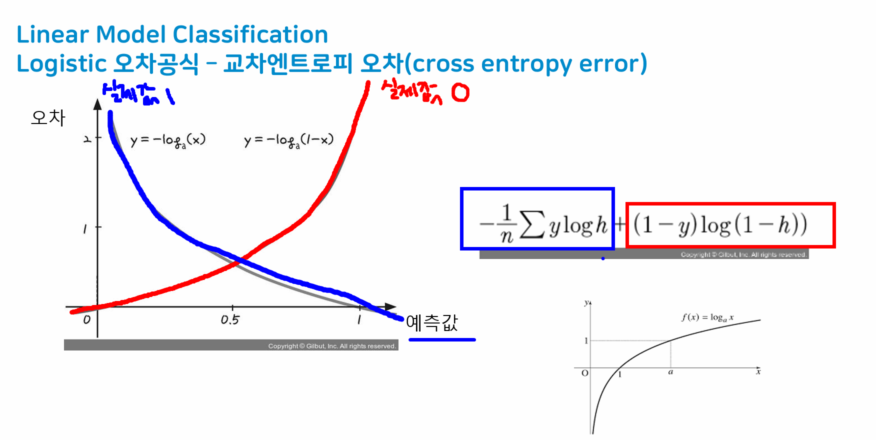
- 오차가 크면 많이 수정하기 때문에 오차를 어떻게 반영해서 수정해나갈 것인지가 포인트
- mse의 경우 분류데이터에는 잘 맞지 않음
- loss function
- 회귀: MSE(평균제곱오차)
- 분류: Cross Entropy Error(교차 엔트로피 오차)
- 분류모델은 다 cross_entropy 씀
분류에서 오차 공식으로 mse를 사용할 경우 ★★★
-
오차가 상대적으로 작게 느껴져 문제가 될 수 있음
-
예시: 타이타닉 생존 여부 예측(label 0, 1)
y 1 1 0 0 1 1 0 1 1 1 0 1
-
→ accuracy: 1/4 = 0.25
→ mse: 3/4 = 0.75 -> 4개 중 3개나 틀린 모델을 0.75만큼만 수정한다는 의미
: mse는 많이 틀리면(오차 크면) 많이 수정해야 하고 오차 작으면 조금만 수정함 → 오차를 크게 보기 위해 제곱하는 건데 1은 제곱해도 1이라 오차가 작게 느껴짐
SVM (Support Vector Machine)
- N차원 공간에서 각 클래스 간의 거리를 최대화하는 최적의 선 또는 초평면을 찾아 데이터를 분류하는 지도형 머신 러닝 알고리즘
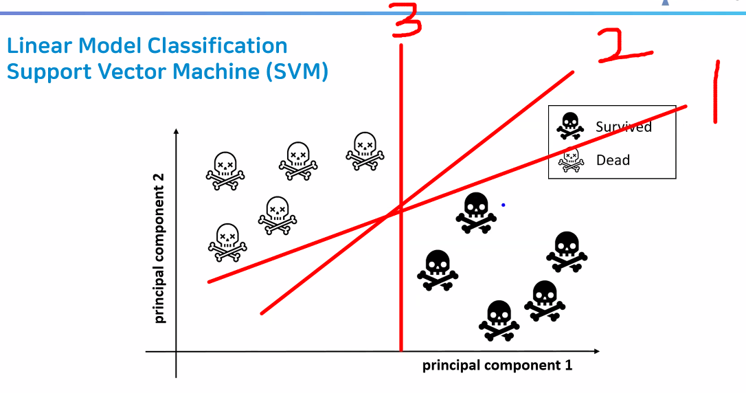
- 선형 분류 모델은 "결정 경계" 역할을 한다 → 데이터를 잘 분류해야 함 → 선과 가까이 있는 데이터를 잘 분류하는 게 관건
- 따라서 현재 분류하고자 하는 데이터로부터 가장 거리가 먼 직선을 구해야 함
- 마진이 최대가 되는 직선 찾기
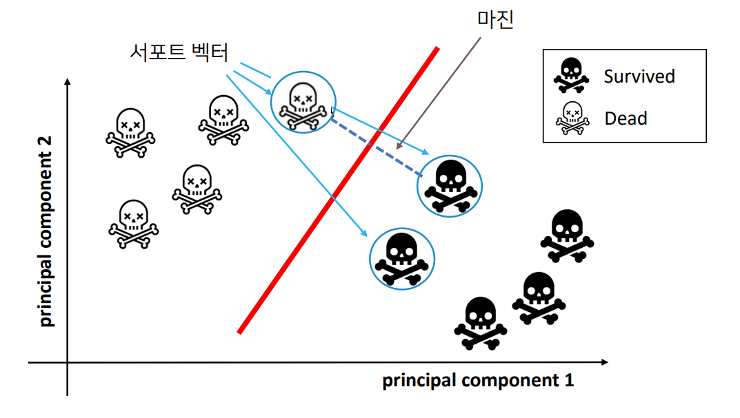
- 서포트 벡터: 서로 반대되는 두 클래스의 가장 가까운 데이터 포인트
- 마진: 서포트 벡터 사이의 거리
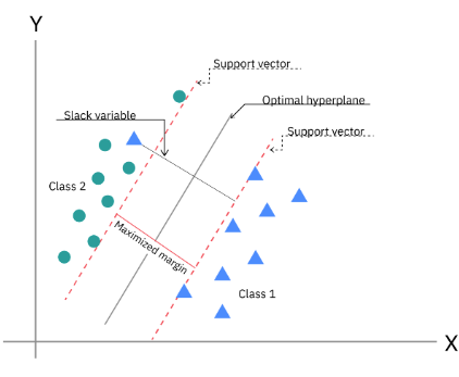
- 마진이 최대가 되는 직선 찾기
장단점
- 선형 모델은 학습 속도가 빠르고 예측도 빠름
- 매우 큰 데이터 세트와 희소(sparse)한 데이터 세트에서도 잘 동작
- 특성이 많을수록 더욱 잘 동작
- 특성이 적은 저차원 데이터에서는 다른 모델이 더 좋은 경우가 많음
실습: 직원 이직 여부 예측
학습 목표
- 선형 분류 모델의 학습 방법에 대해서 알 수 있다.
- 가설 설정을 진행하여 직원의 이직 여부를 예측할 수 있다.
- 분류 평가 지표에 대해 알 수 있다.
1. 문제 정의
- Role: HR 부서 직원
- 직원 이직 여부 데이터 분석을 통해 직원의 이직 여부를 예측해보자
- 이직과 관련 있는 사항들을 지속적으로 확인 후 개선, 직원 관리 프로그램을 운영
- 핵심 인재의 유출을 막아보려 함
- 성과에 따른 보상
- 효율적인 업무 분배
- 쾌적한 환경 등
2. 데이터 수집
- IBM 가상 시나리오 데이터
- 직원 이직 여부 데이터
- IBM HR Analytics Employee Attrition & Performance Dataset에서 확인 가능
# 라이브러리 불러오기
import numpy as np
import pandas as pd
import matplotlib.pyplot as plt
import seaborn as sns

# warning 제거
import warnings
warnings.filterwarnings('ignore')

# 데이터 불러오기
df = pd.read_csv("./data/job_transfer.csv")

# 형태 확인
df.shape
컬럼 설명
| 컬럼명 | 설명 |
|---|---|
| Age | 직원의 나이 |
| Attrition | 이직 여부 (Yes, No) |
| BusinessTravel | 출장을 얼마나 자주 가는지 (Non-Travel, Travel_Rarely, Travel_Frequently) |
| DailyRate | 일일 급여 |
| Department | 부서 (Sales, Research & Development, Human Resources) |
| DistanceFromHome | 집에서 직장까지의 거리 |
| Education | 교육 수준 (1: Below College, 2: College, 3: Bachelor, 4: Master, 5: Doctor) |
| EducationField | 전공 분야 (Life Sciences, Other, Medical, Marketing, Technical Degree, Human Resources) |
| EmployeeCount | 직원 수 (모든 행이 1로 동일) |
| EmployeeNumber | 직원 식별 번호 |
| EnvironmentSatisfaction | 직무 환경 만족도 (1: Low, 2: Medium, 3: High, 4: Very High) |
| Gender | 성별 (Male, Female) |
| HourlyRate | 시간당 급여 |
| JobInvolvement | 직무 몰입도 (1~4) |
| JobLevel | 직무 레벨 (직위 수준) |
| JobRole | 직무 유형 (Sales Executive, Research Scientist, Laboratory Technician, 등) |
| JobSatisfaction | 직무 만족도 (1: Low, 2: Medium, 3: High, 4: Very High) |
| MaritalStatus | 결혼 여부 (Single, Married, Divorced) |
| MonthlyIncome | 월 급여 |
| MonthlyRate | 월 급여 비율 |
| NumCompaniesWorked | 근무했던 회사 수 |
| Over18 | 18세 이상 여부 (모든 값이 Y) |
| OverTime | 초과 근무 여부 (Yes, No) |
| PercentSalaryHike | 급여 인상 비율 (%) |
| PerformanceRating | 성과 평가 (1~4) |
| RelationshipSatisfaction | 동료 및 상사와의 관계 만족도 (1~4) |
| StandardHours | 표준 근무 시간 (모든 값이 80) |
| StockOptionLevel | 스톡옵션 수준 (0~3) |
| TotalWorkingYears | 총 경력 연수 |
| TrainingTimesLastYear | 작년에 받은 교육 횟수 |
| WorkLifeBalance | 워라밸 수준 (1: Bad, 2: Good, 3: Better, 4: Best) |
| YearsAtCompany | 현 회사 근속 연수 |
| YearsInCurrentRole | 현재 직무 근속 연수 |
| YearsSinceLastPromotion | 마지막 승진 이후 경과 연수 |
| YearsWithCurrManager | 현재 매니저와 함께 일한 연수 |
3. 데이터 전처리
- 결측치가 없으므로 따로 전처리 X
4. 탐색적 데이터 분석(EDA)
# 정답 데이터 확인
df["Attrition"].value_counts()

# 이직률 확인
df["Attrition"].value_counts(normalize=True)

sum(df["Attrition"] == "Yes")/len(df["Attrition"])*100
# 16.12% 이직률

# 학습 및 집계함수를 사용하기 위하여 정답 데이터를 수치 데이터로 변경
# 이직: 1, 이직 안 함: 0
# np.where(조건, 조건에 해당 시 반환할 값, 미해당 시 반환할 값)
df["Attrition"] = np.where(df["Attrition"]=="Yes", 1, 0)
df["Attrition"].value_counts()

# 연령 데이터 범주화
np.sort(df["Age"].unique())

# 세분화 되어있는 연령 데이터를 범주화
# 30세 미만, 30세~39세 -> 30대, 40세 이상
df["Age_gp"] = np.where(df["Age"]<30, "30대 미만", np.where(df["Age"]<40, "30대", "40대 이상"))
df["Age_gp"].value_counts()

# 연령대별 이직률 현황
df.groupby("Age_gp")["Attrition"].value_counts()

# 이직률을 어떻게 구할까?
# 이직률 = 이직한 직원 수 / 전체 인원 수 * 100

# 연령대별 이직률 구하는 법
# 1. Age_gp 기준 groupby
# 2. 이직한 직원 수 sum → Attrition이 1이기 때문에 더하면 됨
# 3. 전체 인원 수 count
df_gp = df.groupby("Age_gp")["Attrition"].agg(["count", "sum"])
df_gp["ratio"] = round((df_gp["sum"]/df_gp["count"])*100, 1)
df_gp["ratio"].sort_values(ascending=False)

# 나이가 어릴수록 이직률이 높아진다!

# 성별에 따른 이직률 현황
df_gd = df.groupby("Gender")["Attrition"].agg(["count", "sum"])
df_gd["ratio"] = round((df_gd["sum"]/df_gd["count"])*100, 1)
df_gd.sort_values(by="ratio", ascending=False)

# 해석:
# 남자에 비해 여자의 이직률이 낮은 편

# 컬럼에 따라 이직률 현황 -> 유의미한 결과가 나올 수 있는 컬럼 찾기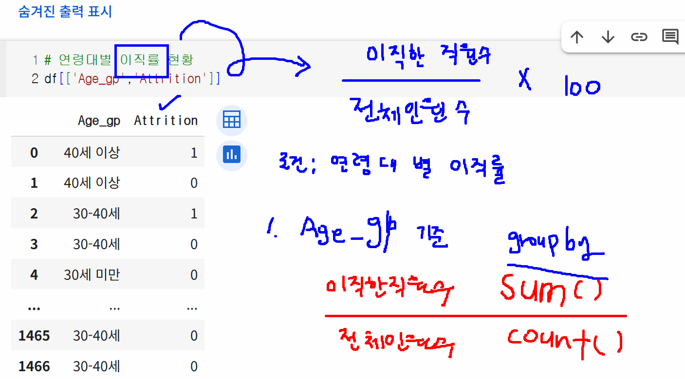
-
유의미한 결과가 있어 보이는 컬럼
- MaritalStatus
- BusinessTravel
- WorkLifeBalance
- JobSatisfaction
- Distance -> 그룹핑 후 관찰
- NumCompaniesWorked 등
-
point
- np.where() 함수를 이용한 범주화
- np.where(조건, 조건에 해당 시 반환할 값, 미해당 시 반환할 값)
- count(): 전체 데이터 수
- sum(): 이진분류 클래스에서 1인 값만 더함 == 이직한 사람 수
- np.where() 함수를 이용한 범주화
가설을 세워 이직률이 높은 데이터를 낮게 제어하기
가설 1
- 업무 만족도(JobSatisfaction)은 높으나 인간 관계 만족도(RelationshipSatisfaction)로 인한 이직률이 높을 것이다.
# 인간 관계 만족도, 업무 만족도 컬럼 가져오기 -> 숫자가 클수록 만족도가 높음
df[["RelationshipSatisfaction", "JobSatisfaction", "Attrition"]].head()

# 인간 관계 만족도, 업무 만족도에 따른 이직률 확인
df_eda = df.groupby(["RelationshipSatisfaction", "JobSatisfaction"])["Attrition"].agg(["count", "sum"])
df_eda["ratio"] = round((df_eda["sum"]/df_eda["count"])*100, 1)
df_eda["ratio"]

# 인간관계 만족도가 높다고 하여 이직률이 적은 것은 아님
# 업무만족도가 높은 직원은 인간 관계에 영향을 덜 받는다
# 업무만족도가 낮은 직원은 인간 관계가 나쁠수록 이직률이 증가하는 경향을 보인다~

# 업무만족도를 높여주는 것이 더 효과적이겠다!- conclusion: 가설 1 기각
- 업무 만족도가 높으면 인간 관계는 큰 영향을 미치지 않음
가설 2
- 근속년수 대비 같은 업무를 오래 한 비중이 높다면 이직률이 높을 것이다.
- 예상: 그럴 것/오히려 낮을 것/관련 없다
# YearsInCurrentRole: 직원이 현재 역할에서 근무한 기간
# YearsAtCompany: 직원이 현재까지 근무한 기간
df[["YearsInCurrentRole", "YearsAtCompany"]]

# 현재 회사는 업무의 변경이 적은 편 -> 적으니까 이직을 많이 하지 않을까?

# 근속년수 대비 한 가지 업종에서 업무를 한 비중
df["Role_Company"] = df["YearsInCurrentRole"]/df["YearsAtCompany"]
df["Role_Company"].fillna(0, inplace=True)
df["Role_Company"]
# 0 / 0은 연산 X -> NaN 출력 -> 0으로 대체(fillna(0))

# 분포와 밀도를 확인
plt.subplots()
sns.distplot(x=df["Role_Company"])
plt.show()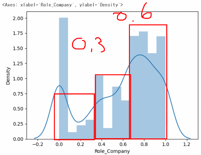
# Role_company 값을 범주화: 0.4 미만, 0.4 이상 0.7 미만, 0.7 이상
# cut은 bin 지정해 줘야 하고 좀 복잡한데 where는 조건만 넣으면 됨
df["Role_Company_gp"] = np.where(df["Role_Company"]<0.4, "0.4 미만", np.where(df["Role_Company"]<0.7, "0.4 이상 0.7 미만", "0.7 이상"))

df["Role_Company_gp"].unique() # NaN이 남아 있지 않은지 확인용

# 근속년수 대비 같은 일을 오래 한 경우 이직률이 낮다 -> 위 범주에 대한 이직률 확인
df_eda = df.groupby("Role_Company_gp")["Attrition"].agg(["count", "sum"])
df_eda["ratio"] = round((df_eda["sum"]/df_eda["count"])*100, 1)
df_eda.sort_values(by="ratio", ascending=False)

# 근속년수 대비 동일한 업무를 오래 한 경우 이직률이 낮다!- Q. 상관계수를 보고 하면 안 되나요?
- A. 상관계수는 숫자 데이터만 확인 가능 & 1대 1로만 상관관계 보여줌 → 우리가 현재 보고자 하는 건 3개 사이의 관계: 여러 개를 연동해서(연결해서) 볼 때는 상관계수가 적합하지 않음
- 정답 데이터에 영향을 주는 컬럼을 추출할 때에는 활용 가능
df.corr(numeric_only=True)["Attrition"].abs().sort_values(ascending=False)흩어져 있는 연속형 데이터들의 분포를 확인할 때 그래프를 그려주면 좋음 → violin plot, distplot, histogram, …
도수분포표와 히스토그램, distplot
- 도수분포표: 범주형 데이터들이 나타내는 빈도수를 정리해 놓은 표
- 데이터 Score(12개): 2, 20, 38, 56, 34, 79, 95, 86, 92, 64, 82, 100
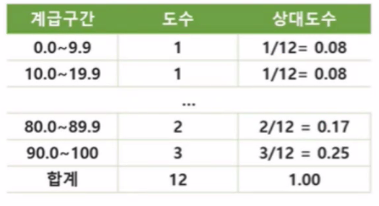
- 데이터 Score(12개): 2, 20, 38, 56, 34, 79, 95, 86, 92, 64, 82, 100
- 히스토그램: 도수분포표를 그래프로 나타낸 것
- 구간별 빈도수를 나타내는 막대 그래프
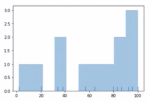
- 구간별 빈도수를 나타내는 막대 그래프
- distplot
- seaborn plot 중 distribution을 표현하는 plot 중 하나
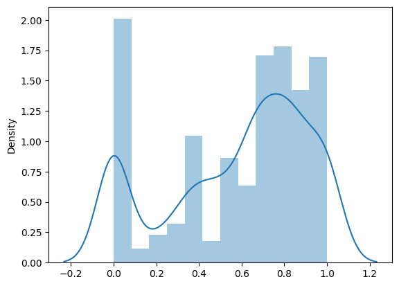
- 파란 선을 없애고 싶다면 kde=False 옵션 주기
- bins 옵션: 간격 나누기
- seaborn plot 중 distribution을 표현하는 plot 중 하나
- 추가: Jointplot
- scatter와 bar를 합치고 싶을 때
- data로 데이터를 주고 x축, y축에 표기할 데이터를 각각 넘기면 됨
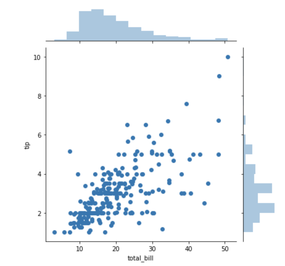
- kind 옵션을 통해 모양 변화 가능(e.g. kind="hex", kind="reg", kind="kde")
- 추가: Pairplot
- 각각 쌍의 그래프를 보여줌
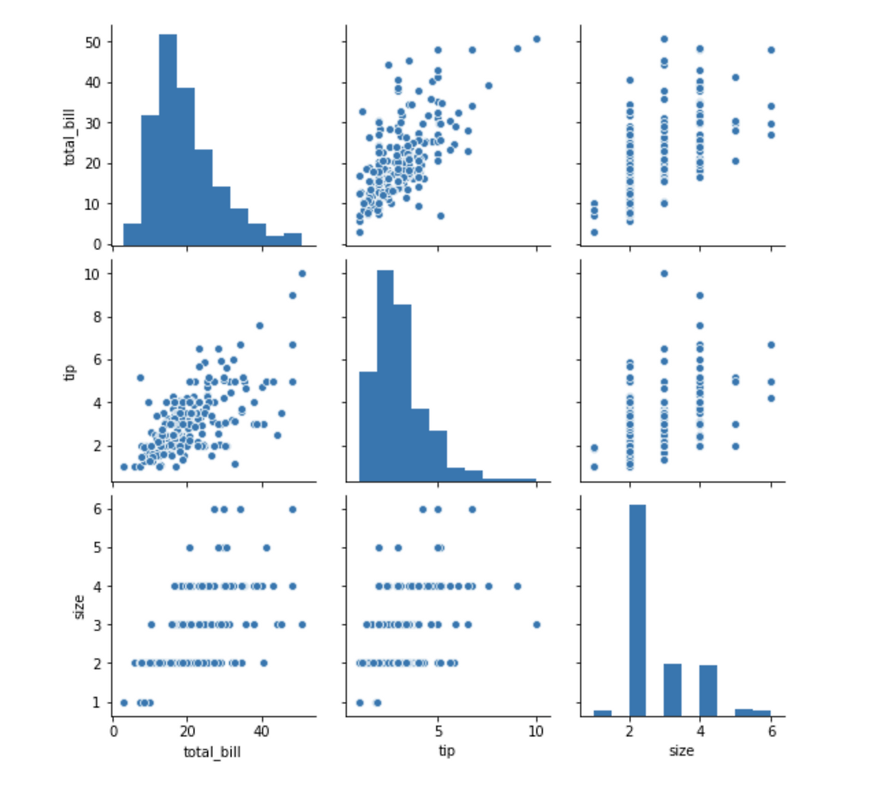
- hue 설정 가능
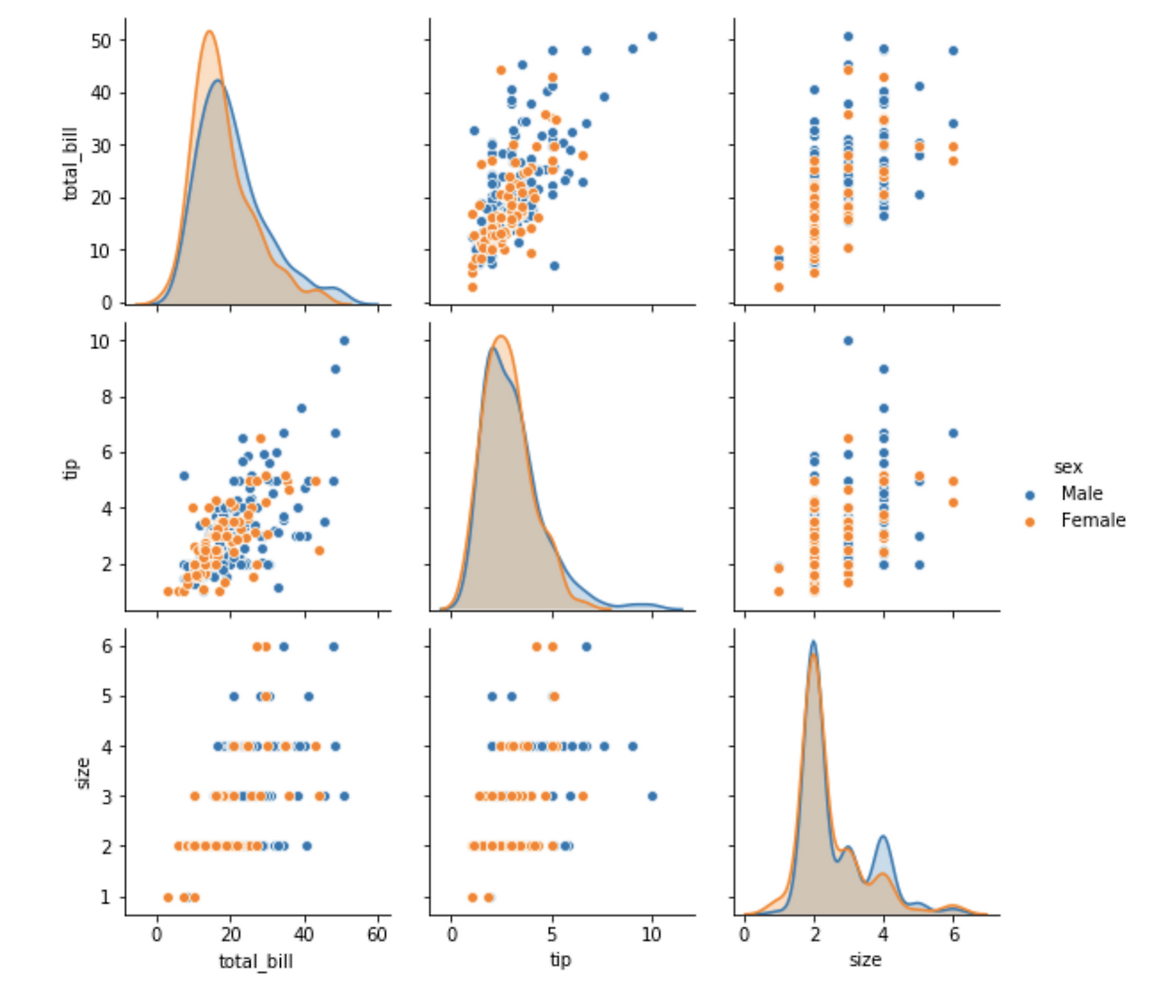
- 각각 쌍의 그래프를 보여줌
- 추가: rugplot
- 각각의 밀도를 보여줌
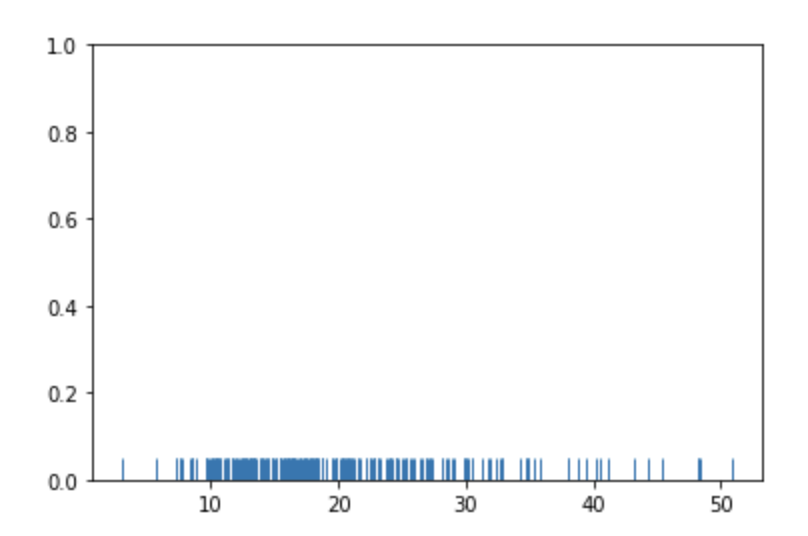
- 밀도가 높은 것이 크기가 큰 데이터이다.
- 각각의 밀도를 보여줌
가설 3
- 야근을 많이 한 사람은 이직률이 높다.
# 계속 쓸 거니까 함수로 만들었음
def get_attrition_ratio(df, *args):
    # args가 1개이고, 그 값이 리스트/튜플이면 풀어서 전달
    if len(args) == 1 and isinstance(args[0], (list, tuple)):
        group_cols = args[0]
    else:
        group_cols = list(args)
    df_eda = df.groupby(group_cols)["Attrition"].agg(["count", "sum"])
    df_eda["ratio"] = round((df_eda["sum"]/df_eda["count"])*100, 1)
    return df_eda["ratio"].sort_values(ascending=False)

# 야근 여부에 따른 이직률 현황
get_attrition_ratio(df, "OverTime")
# 야근을 많이 할수록 이직률이 높다!

# PercentSalaryHike: 연봉인상률
get_attrition_ratio(df, "OverTime", "PercentSalaryHike")

# 야근 Yes 사람들의 이직률 평균 확인
# 야근 Yes 직원 Data 분석 -> 연봉인상률(x)에 따른 이직률 (y)
df_gp_plot = get_attrition_ratio(df, "OverTime", "PercentSalaryHike").reset_index()
df_gp_yes = df_gp_plot[df_gp_plot['OverTime'] == 'Yes']

plt.subplots()
sns.barplot(data=df_gp_yes, x="PercentSalaryHike", y="ratio")
plt.ylim(10,)
plt.show()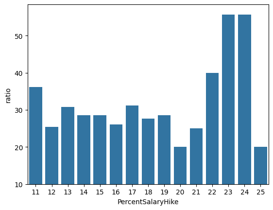
하루 돌아보기
👍 잘한 점
- 가설 2개 제출
- 보충 추업(파이썬 라이브러리 복습) 참여
- 야간자율학습 진행
👎 아쉬웠던 점
- 녹화본이 제공된다는 생각에 집중을 덜 해서 설명을 놓치고 지나간 부분이 있음
- 실습과 이론 설명을 번갈아가면서 하시는 걸 그대로 따라가며 작성하고 있는데 이렇게 쓰니까 나중에 해당 내용을 찾아볼 때 좀 어려움
🔬 개선점
- 수업 시간에 집중하기
- 메모 작성법 익혀서 효율적인 기록 습관 들이기
- 블로그 참고해서 내용 정리하기
- GitHub를 이용해 새 블로그 만드는 중 → 조급해 하지 말고 차근차근 옮기기

2 B R 0 2 B