[인공지능사관학교: 자연어분석A반] 딥러닝 (3)

Suhyeon Lee·2025년 7월 15일

인공지능사관학교

코딩테스트 연습

알고리즘

SQL

지난 시간 복습

딥러닝이란?
- 인간의 신경망(뉴런)을 모방하여 데이터를 학습 및 예측, 평가하는 기술
퍼셉트론(Perceptron)
- 딥러닝 신경망을 구성하는 가장 작은 단위
- 퍼셉트론 = 선형모델 + 활성화함수(P = Linear + Activation)
- 단층 퍼셉트론 → XOR 문제
다층 퍼셉트론(MLP, Multi Layer Perceptron)
- layer 증가할수록 과대적합 주의

모델링
1. 모델 구조 설계
  - 뼈대 생성(Sequential)
  - 입력층(Input(shape=())) → 입력받는 데이터의 형태를 지정: 2차원 데이터는 (컬럼 개수, ) / 이미지 데이터는 (가로 픽셀 수, 세로 픽셀 수)
  - 중간층(Dense(units=?, activation=?)) → 모델의 학습 성능을 설정
  - 출력층(Dense(units=?, activation=?)) → 출력하고자 하는 데이터의 형태를 설정
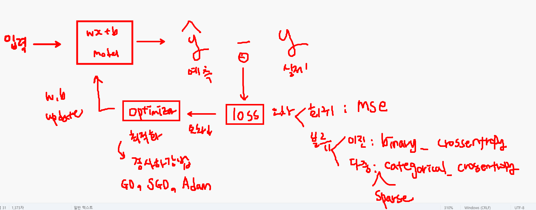
2. 모델 학습 방법 및 평가 방법 설정 (compile)
  - loss: 학습에 사용하는 오차 종류
  - optimizer: 최적화 알고리즘(오차를 줄여나가는 방법 중 하나로 최적의 w, b값을 찾는다. e.g. 경사하강법)
  - metrics: 평가 지표
3. 모델 학습(fit)
  - 데이터: X_train, y_train
  - epochs: 반복 학습 횟수
  - validation_split: 검증 데이터의 비율
  - batch_size: 데이터를 한 번에 학습에 사용하지 않고 나누는 크기(디폴트 값은 32, 일반적으로 32나 64 사용)
  
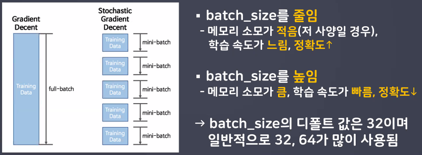
  → 모델 학습할 때 Epoch 1/20 밑에 1500/1500으로 나오는 게 batch size임: $(60000*0.8)/32 = 1500$
4. 시각화
  - loss, val_loss 비교
  - 오차가 학습이 진행될수록 줄어들어야 제대로 된 학습을 했다고 봄
  - 만약에 val_loss가 갑소하다가 증가 → 과대적합의 위험이 있을 수 있다 → 과대적합 제어: 모델 복잡도 낮추기(층, 퍼셉드론 수 ↓), 데이터 많이 수집하기
5. 모델 예측 및 평가(predict, evaluate)

활성화함수 → 추가연산 담당: 중간층에서의 역할과 출력층에서의 역할이 다름!
- 중간층: 활성화/비활성화 여부
  (== 역치 → 반응을 위한 최소 자극)
  - 인간의 역치 개념을 가져오기 위해 초기에는 계단 함수(step function) 사용 → optimizer에서 미분 시 기울기 문제 발생 → 시그모이드(sigmoid) 사용 → 층이 많아지고 퍼셉트론의 수가 많아지면 역전파 과정에서 기울기 소실 문제(vanishing gradient) 발생 → ReLU 사용
- 출력층: 출력하고자 하는 데이터의 형태를 설정
  - 회귀: linear(항등함수, y=x) → 선형모델이 예측한 결과를 그대로 출력 → 디폴트 값이라 따로 적지 않아도 됨
  - 이진분류: sigmoid → 선형모델이 예측한 결과(-∞ ~ ∞로 뻗어 나가는 연속형 데이터)를 0~1 사이의 확률 값으로 변환(변환 결과가 0.5 이상이면 class 1)
  - 다중분류: softmax → 선형모델이 예측한 결과를 총합이 1인 확률 값으로 변환(확률 값은 class 개수만큼 나옴)

출력층 units 개수 설정
- 회귀: 1개(units=1) → 수치형 결과 1개
- 이진분류: 1개(units=1) → 1개의 확률값을 출력받기 위함
- 다중분류: class 개수만큼(units=클래스 개수) → 클래스 개수만큼의 확률 값(연속적인 숫자로 표현됨) 출력받고자 하기 때문

학습 방법 및 평가 방법 예측(compile)
- loss: 손실 함수 → 오차(실제값과 예측값의 차이)
  - 회귀: mean_squared_error
  - 이진분류: binary_crossentropy
  - 다중분류: categorical_crossentropy → 정답 데이터와 출력 데이터의 차원이 일치하지 않을 경우 sparse_categorical_crossentropy
- optimizer: 최적화함수 → 오차를 줄여나가는 방법 정의
  - 경사하강법(GD), SGD, Adam
- metrics: 평가 지표
  - 회귀: mse(평균제곱오차)
  - 분류: accuracy(정확도)

실습: 다양한 조합으로 모델링

학습 목표

손글씨 데이터를 활용해 다양한 활성화 함수와 경사하강법 조합을 하여 모델의 성능을 비교해보자.

모델 조합

model1
- sigmoid + SGD 조합
model2
- relu + SGD 조합
model3
- relu + Adam 조합
모델 설계, 학습, 시각화
- 모델 1, 2, 3의 결과를 하나의 그래프에 출력
단, 모델 설계 시 5층 쌓기
- 64, 128, 256, 128, 64
학습 횟수: 20
검증 데이터 20% 사용

은닉층: 항아리 모양

units를 64 → 128 → 256 → 128 → 64로 늘렸다가 줄이는 과정을 통해 특성을 더 잘 추출할 수 있다는 특징이 있음

import numpy as np
import pandas as pd
import matplotlib.pyplot as plt

from tensorflow.keras.datasets import mnist
from tensorflow.keras import Sequential
from tensorflow.keras.layers import Input, Dense, Flatten
from tensorflow.keras.optimizers import SGD, Adam

(X_train, y_train), (X_test, y_test) = mnist.load_data()

# 모델 1: sigmoid + SGD
model1 = Sequential()
model1.add(Input(shape=(28,28)))
model1.add(Flatten())
model1.add(Dense(units=64, activation='sigmoid'))
model1.add(Dense(units=128, activation='sigmoid'))
model1.add(Dense(units=256, activation='sigmoid'))
model1.add(Dense(units=128, activation='sigmoid'))
model1.add(Dense(units=64, activation='sigmoid'))
model1.add(Dense(units=10, activation='softmax'))
model1.compile(
    optimizer=SGD()
    , loss="sparse_categorical_crossentropy"
    , metrics=["accuracy"]
)
h1 = model1.fit(X_train, y_train, validation_split=0.2, epochs=20, batch_size=64)

# 모델 2: : ReLU + SGD → default 값으로 학습 시 보폭이 너무 커 제대로 학습하지 못함 → 하이퍼 파라미터 조정
model2 = Sequential()
model2.add(Input(shape=(28,28)))
model2.add(Flatten())
model2.add(Dense(units=64, activation='relu'))
model2.add(Dense(units=128, activation='relu'))
model2.add(Dense(units=256, activation='relu'))
model2.add(Dense(units=128, activation='relu'))
model2.add(Dense(units=64, activation='relu'))
model2.add(Dense(units=10, activation='softmax'))
model2.compile(
    optimizer=SGD(learning_rate=0.001) # 0.01일 때 loss가 None으로 출력됨 → learning rate=0.01이 너무 높다는 뜻
    , loss="sparse_categorical_crossentropy"
    , metrics=["accuracy"]
)
h2 = model2.fit(X_train, y_train, validation_split=0.2, epochs=20, batch_size=64)

# 모델 3: ReLU + Adam
model3 = Sequential()
model3.add(Input(shape=(28,28)))
model3.add(Flatten())
model3.add(Dense(units=64, activation='relu'))
model3.add(Dense(units=128, activation='relu'))
model3.add(Dense(units=256, activation='relu'))
model3.add(Dense(units=128, activation='relu'))
model3.add(Dense(units=64, activation='relu'))
model3.add(Dense(units=10, activation='softmax'))
model3.compile(
    optimizer=Adam() # Adam의 default learning_rate는 0.001 cf. SGD는 default 0.01
    , loss="sparse_categorical_crossentropy"
    , metrics=["accuracy"]
)
h3 = model3.fit(X_train, y_train, validation_split=0.2, epochs=20, batch_size=64)

# 시각화: accuracy
plt.figure(figsize=(8,3))
plt.plot(h1.history["accuracy"], label="sig+sgd acc")
plt.plot(h2.history["accuracy"], label="relu+sgd acc")
plt.plot(h3.history["accuracy"], label="relu+adam acc")
plt.plot(h1.history["val_accuracy"], label="sig+sgd acc_val")
plt.plot(h2.history["val_accuracy"], label="relu+sgd acc_val")
plt.plot(h3.history["val_accuracy"], label="relu+adam acc_val")
plt.legend()
plt.show()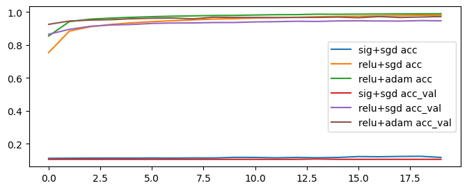

# 시각화: loss
plt.figure(figsize=(8,3))
plt.plot(h1.history["loss"], label="sig+sgd loss")
plt.plot(h2.history["loss"], label="relu+sgd loss")
plt.plot(h3.history["loss"], label="relu+adam loss")
plt.plot(h1.history["val_loss"], label="sig+sgd loss_val")
plt.plot(h2.history["val_loss"], label="relu+sgd loss_val")
plt.plot(h3.history["val_loss"], label="relu+adam loss_val")
plt.legend()
plt.show()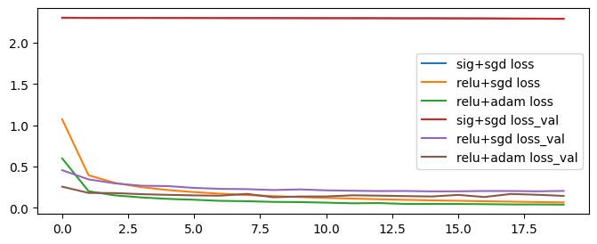

서로에게 맞는 최적화 함수와 활정화 함수가 있음!
→ 다양한 조합과 다양한 파라미터로 학습을 진행하기

callback 함수

모델 저장
- 학습을 완료한 모델 저장 (중간 저장 가능)
- modelcheckpoint
  - 딥러닝 모델 학습 시 저장된 epoches를 모두 진행하면 과대적합이 되는 경우가 있음 → 중간에 일반화된 모벨을 저장
  - 커널이 끊기면 정보가 날아가기 때문에 학습 내용을 저장
조기 학습 중단
- 모델의 성능이 더 이상 향상되지 않을 때 학습을 조기에 중단시킬 수 있음
- earlystopping
  - epochs를 크게 설정한 경우 일정 횟수 이후로는 모델의 성능이 크게 개선되지 않는 경우가 있음
  - 모델의 성능이 더 이상 개선되지 않을 때 조기 학습 중단

모델을 학습할 때 학습 중간에 프로그램이 오류가 난다면 지금까지 학습했던 가중치를 모두 잃게 되는 일이 발생합니다.
모델을 학습 중간마다 저장하면 프로그램이 끊기더라도 체크포인트부터 다시 시작할 수 있습니다.
- 텐서플로우 콜백 함수를 이용해 모델을 중간 저장하고 다시 로드해서 학습힐 수 있습니다.

모델을 중간 중간 저장하는 습관 들이기

from tensorflow.keras.callbacks import ModelCheckpoint, EarlyStopping

# 모델 저장
# 경로 설정
model_path = "/content/drive/MyDrive/Colab Notebooks/DeepLearning_basic/data/model_save/model_{epoch:02d}_{val_accuracy:.3f}.keras"

# 모델 저장 객체 생성 → 학습할 때 사용
mc = ModelCheckpoint(
    filepath=model_path # 모델을 저장할 경로
    , monitor="val_accuracy" # 모델의 성능을 확인하는 기준(최고점(최고 성능) 판단 기준)
    , verbose=1 # 진행 과정 출력 여부(0→미출력, 1→출력)
    , save_best_only=True # 모델이 최고 성능을 갱신할 때만 저장 (False → 모든 epoch마다 저장): 메모리를 아끼기 위해서 꼭 True로
)

# 조기학습 중단 객체 생성
es = EarlyStopping(
    monitor="val_accuracy" # 중단할 기준
    , verbose=1 # 로그 출력 여부
    , patience=20 # 모델 성능 개선을 기다리는 횟수
)

# 모델 1: sigmoid + SGD
model1 = Sequential()
model1.add(Input(shape=(28,28)))
model1.add(Flatten())
model1.add(Dense(units=64, activation='sigmoid'))
model1.add(Dense(units=128, activation='sigmoid'))
model1.add(Dense(units=256, activation='sigmoid'))
model1.add(Dense(units=128, activation='sigmoid'))
model1.add(Dense(units=64, activation='sigmoid'))
model1.add(Dense(units=10, activation='softmax'))

# 학습 방법
model1.compile(
    optimizer=SGD()
    , loss="sparse_categorical_crossentropy"
    , metrics=["accuracy"]
)

# 학습
h1 = model1.fit(
    X_train
    , y_train
    , validation_split=0.2
    , epochs=100
    , batch_size=64
    , callbacks = [mc,es]
)

# 콜백 함수를 사용한 결과 → acc, val_acc 그래프 그려보기
plt.figure(figsize=(10,6))
plt.plot(h1.history["accuracy"], label="acc")
plt.plot(h1.history["val_accuracy"], label="val_acc")
plt.show()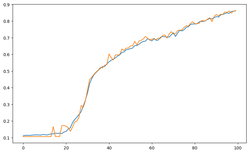

추가: 모델 불러오기

from tensorflow.keras.models import load_model
model_loaded = load_model("/content/drive/MyDrive/Colab Notebooks/DeepLearning_basic/data/model_save/model_89_0.890.keras")
model_loaded.summary()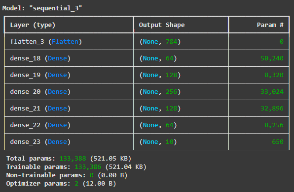

Pytorch 맛보기

학습 목표

Pytorch 사용을 위한 환경 설정을 진행하고 텐서(Tensor)에 대한 개념에 대해 알 수 있다.
Pytorch의 다양한 사용법에 대해 알 수 있다.

Pytorch?

Facebook(현 Meta)에서 개발한 오픈소스 딥러닝 프레임워크
초기에 토치는 넘파이 라이브러리처럼 과학 연산을 위한 라이브러리로 공개
- 토치는 루아(Lua, EncodeLua)로 개발 → 파이썬 버전으로 만듦: Pytorch
GPU를 이용한 텐서 조작 및 동적신경망 구성이 가능하도록 딥러닝 프레임워크로 발전

사용 분야

자연어 처리(NLP)
이미지 처리(컴퓨터비전)
시계열 예측
생성형 모델

Pytorch vs. Keras

Keras는 사용자 친화적: block coding에 가까움(모듈화)
- 직관적인 API와 쉬운 사용법 → 딥러닝 모델 구축이 간편
- 모듈 형태의 구성 요소 → 새 모델을 만들 때 각 모듈을 조합해 쉽게 새로운 모델 생성 가능
Pytorch는 커스터마이징에 강점
- 딥러닝 모델을 만드는 데 기초 레벨부터 직접 작업
- 유연성 및 제어 용이성: 저수준 연산에 대한 접근이 용이하여 복잡한 모델이나 연구 목적에 적합
- 예: huggingface에 올라온 모델 → 내 데이터에 그대로 사용할 수 없음: 커스터마이징 필수! → Pytorch를 사용하는 게 훨씬 유용
더 알아보기

환경 설정

PyTorch documentation
- PyTorch is an optimized tensor library for deep learning using GPUs and CPUs.
  - using GPUs and CPUs → 빠른 연산 가능
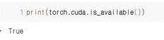
cuda 사용 가능 여부 확인
- cuda: 엔비디아(NVIDIA)에서 만든 GPU 컴퓨팅 기술
- 딥러닝 연산을 GPU에서 처리하겠다는 의미
- 구글 colab에서는 런타임 유형 변경 > 하드웨어 가속기를 T4 GPU로 변경하면 cuda 이용 가능
  - 하지만 GPU 사용량 한도에 도달하지 않도록 GPU를 활용하지 않는 경우 표준 런타임으로 전환하는 것이 좋음 (오늘 진행할 실습에서는 꺼 두기)

# 설치 확인 및 버전 확인
import torch, torchvision

print(torch.__version__)
print(torchvision.__version__)
print(torch.cuda.is_available()) # 구글 코랩 기본 설정은 CPU라 런타임 유형 설정 안 바꾸고 하면 False가 뜹니다.

# 컴퓨팅 자원을 아껴두기 위해 CPU로 설정하고 진행해 주세요.

2.6.0+cu124
0.21.0+cu124
False

하드웨어 가속기를 T4 GPU로 변경하면:

기본 구성 요소

Tensor, Autograd, nn.Module, Dataset & DataLoader

텐서(Tensor)

다차원 배열 구조
파이토치(Pytorch)의 기본 데이터 구조
- 파이토치는 데이터 표현을 위한 기본 구조로 Tensor를 사용함
- cf. 넘파이는 ndarray, 판다스는 Series와 DataFrame
- 데이터와 gradient 계산을 위한 메타네이터를 포함하고 있음
넘파이 배열과 유사하지만, GPU 연산 가속 가능
- 가속 연산이 가능하기 때문에 넘파이 배열이 아닌 텐서를 사용해 딥러닝 진행
텐서는 모든 딥러닝 연산의 기본 단위
딥러닝 모델의 입출력 구조를 이해하기 위해 필요
- 입력 텐서의 모양을 정확히 알아야 Linear, Conv 등 층 설계에 도움이 된다!
속성
- data
  - 텐서의 주요 구성 요소
  - 실제 수치 정보를 저장
  - 데이터는 다양한 차원을 가질 수 있으며, 신경망에서는 주로 벡터, 행렬 또는 더 높은 차원의 배열로 사용
- dtype
  - 텐서에 저장된 데이터 타입을 정의( 'torch.float32'; 'torch.int64' 등)
- device
  - 텐서가 어떤 장치(CPU,GPU)에 할당되어 있는지 나타냄
- requires_grad
  - 해당 속성이 'True'로 설정되어 있으면, 텐서에 대한 모든 연산이 자동 미분 시스템에 의해서 추적됨 → 이를 통해 gradient가 자동으로 계산: 학습과정에서 매우 중요한 요소
- grad
  - equires_grad가 'True'로 설정된 텐서에 대해 연산이 수행될 때, Pytorch가 자동으로 gradient를 계산하고 이를 grad속성에 저장
  - gradient는 파라미터의 최적화에 사용
- shape
  - 텐서의 차원을 나타내며, 각 차원의 크기(Size)를 포함

import torch

# 텐서 생성
torch.tensor([[1, 2],
              [3, 4]])

tensor([[1, 2],
        [3, 4]])

벡터, 행렬 그리고 텐서(Vector, Matrix and Tensor)
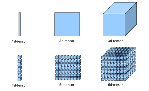
- 딥 러닝을 위한 가장 기본적인 수학적 지식인 벡터, 행렬, 텐서의 개념에 대해서 이해하고, Numpy와 파이토치로 벡터, 행렬, 텐서를 다루는 방법에 대해서 이해하기
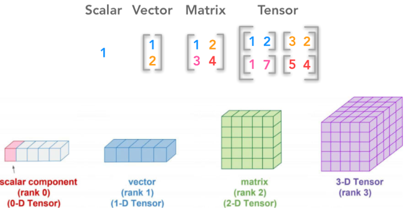
- 딥 러닝의 기본 단위: scalar, vector, matrix, tensor
  - scalar(0d-tensor): 기본 변수 (숫자 하나) → 차원이 없는 값
  - vector(1d-tensor): 1차원 배열
  - matrix(2d-tensor): 2차원 배열
  - tensor(3d-tensor): 3차원 이상의 tensor를 의미 (텐서는 차원이라고 생각하면 편해요!)

3차원 Tensor

세로, 가로, 깊이
- 테이블(표) 데이터
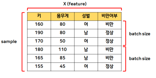
  - (특성, 데이터 수, 샘플링 수)
- 이미지 데이터 세트
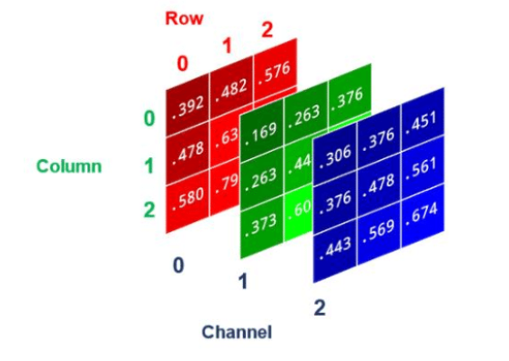
  - (가로, 세로, 색상 채널) → 색상 채널이 1: 흑백, 색상 채널이 3: RGB
- 문장 데이터 세트
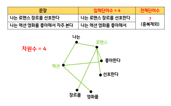
  - (입력 문장 수, 전체 단어 수, 차원 수) → [2, 4, 4]

Pytorch Tensor 자료형

torch.Tensor 클래스에 대한 심층적인 소개
공식 문서: torch.Tensor
- A torch.Tensor is a multi-dimensional matrix containing elements of a single data type.

PyTorch 타입 이름	실제 자료형(dtype)	설명
`FloatTensor`	`torch.float32`	32비트 실수형(32-bit floating point)
`DoubleTensor`	`torch.float64`	64비트 실수형
`HalfTensor`	`torch.float16`	16비트 실수형
`BFloat16Tensor`	`torch.bfloat16`	16비트 실수형
`IntTensor`	`torch.int32`	32비트 정수형
`LongTensor`	`torch.int64`	64비트 정수형
`ShortTensor`	`torch.int16`	16비트 정수형
`CharTensor`	`torch.int8`	8비트 정수형
`ByteTensor`	`torch.uint8`	8비트 부호 없는 정수형
`BoolTensor`	`torch.bool`	Boolean

torch.FloatTensor의 별칭: torch.Tensor
- 기본적으로 PyTorch tensor는 32-bit 부동 소수점 표현 실수로 채워짐
  - GPU에서 사용하는 tensor는 float32가 가장 최적화되어 있음
- 하지만 모델에 따라 특정 조건(규칙)이 있을 때가 있어(예: 출력층에서 이진분류 설계 시 반드시 LongTensor여야 함) 타입을 모두 알아두는 게 좋음
이 외에도 complex, quantized 등이 존재

BF16(bfloat16, Brain Floating Point)
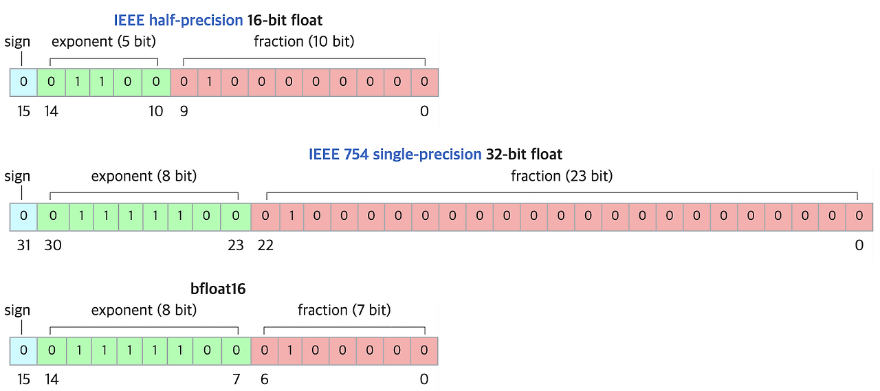
- 자릿수를 대표하는 지수항(exponent)에 할당한 bit가 FP32와 동일한 8개
  - 수의 표현 범위를 FP32와 동등한 수준으로 만듦 (최댓값: 65536 → 약 $2^{128}$ )
  - 더 넓은 범위의 수를 표현할 수 있는 대신 수의 표현 정밀도가 떨어짐
    - 장점: 넓은 수의 표현 범위
    - 단점: 표현 정밀도가 떨어지기 때문에 0에 가까운 수가 모두 0으로 표현될 수 있음 → 계싼을 하다가 어떤 수를 0으로 나누는 상황이 생길 가능성을 높임

실습

# 실수형 텐서 생성
t_float = torch.FloatTensor([[1, 2], [3, 4]])
t_long = torch.LongTensor([[1, 2], [3, 4]])
print(t_float.dtype)
print(t_long.dtype)

torch.float32
torch.int64

원하는 크기의 임의의 값을 갖는 텐서 생성: torch.rand(), torch.randn()
- numpy에서는 특정 값으로 배열 생성 시 np.ones, np.zeros 등, 임의의 값으로 배열 생성 시 np.random.rand 등을 사용했었음

# 32비트 실수형 데이터를 갖는 임의의 텐서 생성
torch.FloatTensor(2, 3) # 메모리에 남아 있던 찌꺼기 값(초기화되지 않은 메모리 값)

tensor([[2.0758e-16, 0.0000e+00, 1.6180e-16],
        [0.0000e+00, 7.0414e-17, 0.0000e+00]])

# 랜덤 값으로 (2,3)의 텐서 생성하기
torch.rand(2,3) # 사용할 수 있는 실수 값 생성

tensor([[0.3889, 0.1263, 0.8998],
        [0.0140, 0.8352, 0.9881]])

요약 비교표

항목	`torch.FloatTensor(2, 3)`	`torch.rand(2, 3)`
값의 의미	초기화되지 않은 메모리 쓰레기값	0 이상 1 미만의 무작위 실수 (균등분포)
난수 생성 여부	❌ 아님 (난수 아님)	✅ 진짜 난수
실전에서의 사용	거의 안 씀 (조심해야 함)	자주 씀 (초기화, 랜덤 샘플 등)

# 정규분포 난수값을 가지는 텐서 생성
torch.randn(2,3)

tensor([[ 1.0045, -1.1222,  0.1809],
        [-0.4668,  0.3108,  1.5698]])

cf. 넘파이

# numpy에서 특정 값으로 배열 생성
import numpy as np

# 1로 채운 넘파이 배열 생성
np.ones((2, 3))

print('np.random.rand\n', np.random.rand(2, 3))
# 0과 1 사이의 균일 분포 난수로 채워진 행렬을 생성
print('np.random.randn\n', np.random.randn(2, 3))
# 표준 정규 분포 (평균 0, 분산 1)를 따르는 난수로 채워진 행렬을 생성
print('np.random.randint\n', np.random.randint(0, 10, size=(2, 3)))
# 지정된 범위 (low 이상 high 미만)의 정수 난수로 채워진 행렬을 생성
print('np.random.choice\n', np.random.choice([1, 2, 3, 4, 5], size=(2, 3), replace=True, p=None))
# 지정된 범위 (low 이상 high 미만)의 정수 난수로 채워진 행렬을 생성
# replace=True는 복원 추출 (중복 허용)을 의미하고, replace=False는 비복원 추출 (중복 불가)을 의미

# cf. 파이썬 random 모듈
import random
print('random.randint\n', random.randint(0, 10))
print('random.sample\n', random.sample(range(1, 101), 5))

np.random.rand
 [[0.05471568 0.2818698  0.20810544]
 [0.87613291 0.51560773 0.35518498]]
np.random.randn
 [[-0.95464116 -0.39966631 -1.39070909]
 [-0.14523821  1.73774026  1.94933784]]
np.random.randint
 [[1 7 6]
 [2 9 2]]
np.random.choice
 [[5 3 4]
 [5 1 4]]
random.randint
 4
random.sample
 [88, 58, 72, 56, 7]

설정한 범위 내에서 정수 난수값을 가진 텐서 생성: torch.randint(), torch.randperm()

# (시작범위, 끝범위+1, 텐서의 크기)
torch.randint(1, 50+1, size=(1,6))

tensor([[42, 17, 20, 19,  9, 33]])

# randperm 함수: 0부터 n-1까지 정수를 하나씩 섞어서 임의의 배열을 생성
# 데이터 세트를 랜덤으로 shuffle
torch.randperm(10)

tensor([1, 9, 3, 4, 2, 5, 0, 8, 7, 6])

pytorch는 numpy와 높은 호환성을 가짐
- torch.from_numpy(arr): numpy를 pytorch tensor로 변경
- torch.tensor.numpy(): pytorch tensor를 numpy로 변경

arr = np.array([[1, 2], [3, 4]])
ten = torch.tensor([[1, 2], [3, 4]])

# ndarray → tensor
torch.from_numpy(arr)

# tensor → ndarray
ten.numpy()

넘파이 배열과 텐서의 장점: 요소별 연산
- 리스트와 다르게 넘파이와 텐서는 "요소별 연산"이 가능하다!

# 리스트
[1, 2, 3] + [1, 2, 3] # 출력: [1, 2, 3, 1, 2, 3]

# 넘파이 ndarray
np.array([1, 2, 3])+np.array([1, 2, 3]) # 출력: array([2, 4, 6])


# 파이토치 tensor
torch.tensor([1, 2, 3])+torch.tensor([1, 2, 3]) # 출력: tensor([2, 4, 6])

타입 변환
- torch.Tensor.long(): long 타입으로 변환
  - cross entropy를 사용하는 출력층에서는 정답 데이터가 무조건 long 타입이어야 함 (규칙임) → 데이터 타입을 long 타입으로 변경해 주는 단계를 거친 후 학습해야 함!
  - Expected object of scalar type Long
- torch.Tensor.float(): float 타입으로 변환
  - 인공신경망에는 정수를 넣을 수 없다는데? 여기서
  - PyTorch models, particularly those involving operations like convolutions, linear layers, and many activation functions, typically expect input tensors to be of a floating-point data type (e.g., torch.float32 or torch.float64). This is because these operations are designed to work with continuous numerical values and often involve calculations that require floating-point precision.

텐서를 확인하는 다양한 키워드
- torch.Tensor.size() 메서드: 데이터의 크기
- torch.Tensor.shape 속성(키워드): 데이터의 형태, 크기
- torch.Tensor.ndim 속성: 데이터의 차원

# (4, 4) 크기로 정규 분포를 갖는 랜덤 텐서 생성
t_randn = torch.randn(4,4)

# 랜덤 텐서 long 형태로 변환
t_long = t_randn.long()
print(t_long)
print(type(t_long))

# 텐서를 numpy로 변환
arr = t_long.numpy()
print(arr)
print(type(arr))

# numpy → 텐서로 변환
ten = torch.from_numpy(arr)
print(ten)
print(type(ten))

# 크기, 차원 출력
print(ten.shape, ten.size(), ten.ndim, sep="\n")

tensor([[ 0,  0,  0,  0],
        [ 0, -1,  0,  1],
        [ 0,  2,  0, -1],
        [ 0,  0,  0,  1]])
<class 'torch.Tensor'>
[[ 0  0  0  0]
 [ 0 -1  0  1]
 [ 0  2  0 -1]
 [ 0  0  0  1]]
<class 'numpy.ndarray'>
tensor([[ 0,  0,  0,  0],
        [ 0, -1,  0,  1],
        [ 0,  2,  0, -1],
        [ 0,  0,  0,  1]])
<class 'torch.Tensor'>
torch.Size([4, 4])
torch.Size([4, 4])
2

# Byte 타입의 5개 크기로 임의의 텐서를 생성하고 랜덤으로 섞는다
# 1. ByteTensor 생성
t_bt=torch.ByteTensor(5)
print(t_bt)
# 2. size 함수를 사용하여 데이터의 개수 파악
s = t_bt.size()
print(s[0])
# 3. torch.randperm을 사용하여 랜덤하게 인덱스 생성
t_idx = torch.randperm(s[0])
print(t_idx)
# 4. torch.randperm이 가지는 숫자를 인덱스로 지정
# 5. 인덱스 번호 순서대로 정렬(인덱싱) → 월화수목금 가져오는 원리와 동일
result = t_bt[t_idx]
print(result)

# 한 줄로도 가능
torch.ByteTensor(5)[torch.randperm(torch.ByteTensor(5).size()[0])]

tensor([ 96, 157, 148,  73, 169], dtype=torch.uint8)
5
tensor([1, 3, 4, 0, 2])
tensor([157,  73, 169,  96, 148], dtype=torch.uint8)

tensor([240,   0,  46,  44,  82], dtype=torch.uint8)

# (3,3) 크기의 임의로 1~10 사이의 정수형 텐서를 생성하고 랜덤으로 섞어서 출력
# 다양한 방법으로 해 보기

# 1. 임의의 3,3 크기의 텐서를 생성 (랜덤 수)
ten_3by3 = torch.randint(1, 10+1, size=(3,3))
print(ten_3by3)
# 2. 반복문을 활용하여 사이즈 추출 (1행, 2행, 3행)
for i in range(ten_3by3.size()[0]):
  idx = torch.randperm(ten_3by3[i].size()[0])
  ten_3by3[i] = ten_3by3[i][idx]
# 3. torch.randperm을 인덱스처럼 활용하여 재배열
# print(임의의 3,3 텐서)
# print(결과)
print(ten_3by3)

# 다른 풀이 1
t_rand = torch.randint(1, 11, size=(3,3))
t_rand_size = t_rand.size() # [3,3]
n_flat = t_rand.numpy().flatten()
row = t_rand_size[0]
col = t_rand_size[1]
n_arr = n_flat[torch.randperm(row*col)]
t_arr = torch.from_numpy(n_arr)
result = t_arr.reshape(row, col)
result

# 다른 풀이 2
data_org = torch.randint(1, 11, (3,3))
print(data_org)
data = data_org.reshape(-1)
idx = torch.randperm(data.shape[0])
data = data[idx]
data = data.reshape(data_org.shape[0], data_org.shape[1])
print(data)

# 다른 풀이 3
t_int = torch.randint(1, 11, (3,3))
print(t_int)
for idx, row in enumerate(t_int):
    size = row.size()
    t_int[idx] = row[torch.randperm(size[0])]
print(t_int)

# 다른 풀이 4
ten_org = torch.randint(1, 10+1, size=(3,3))
print(ten_org)
row_num = ten_org.shape[0]
col_num = ten_org.shape[1]
ten_shuffled = []
for i in range(row_num):
  idx = torch.randperm(col_num)
  ten_shuffled.append(ten_org[i][idx])
ten_shuffled = torch.stack(ten_shuffled)
result = ten_shuffled[torch.randperm(row_num)]
print(result)

# 다른 풀이 5
t_rand3 = torch.randint(1, 10+1, size=(3,3))
print(t_rand3)

rand_rows = t_rand3[torch.randperm(t_rand3.size(0))]
print(rand_rows)

rand_tensor = t_rand3.view(-1)[torch.randperm(9)].reshape(3,3)
print(rand_tensor)

# 강사님 풀이
# (3,3) 크기의 임의로 1~10 사이의 정수형 텐서를 생성하고 / 랜덤으로 섞어서 출력
# 1. 임의의 3,3 크기의 텐서를 생성 (랜덤수)
rand_int = torch.randint(1,11,size=(3,3))
print(rand_int)
# 2. 반복문을 활용하여 사이즈 추출 (1행,2행,3행)
for i in range(rand_int.shape[0]):
    s = rand_int[i].size(0)
    idx = torch.randperm(s)
    rand_int[i] = rand_int[i][idx]
# 3. torch.randperm 을 인덱스처럼 활용하여 재배열
print(rand_int)
# print(임의의 3,3 텐서)
# print(결과)

# 또 다른 방법
t_int = torch.randint(1,11,(3,3))
print('원본')
print(t_int)

for dim in range(t_int.ndim):
    perm = torch.randperm(t_int.size(dim))
    t_int = t_int[perm] if dim == 0 else t_int[:, perm]

print('변환')
print(t_int)

하루 돌아보기

👍 잘한 점

텐서가 이해가 안 되어서 추가 학습 진행 → 정리글

👎 아쉬웠던 점

벨로그 이미지 업로드가 안 되고 있어서 노트 정리를 제대호 못 했음

🔬 개선점

내일 복습하면서 노트 채우기

Suhyeon Lee

2 B R 0 2 B

이전 포스트

[인공지능사관학교: 자연어분석A반] 딥러닝 (2)

다음 포스트

[인공지능사관학교: 자연어분석A반] 딥러닝 (3)

코딩테스트 연습

알고리즘

SQL

지난 시간 복습

실습: 다양한 조합으로 모델링

학습 목표

모델 조합

은닉층: 항아리 모양

callback 함수

추가: 모델 불러오기

Pytorch 맛보기

학습 목표

Pytorch?

사용 분야

Pytorch vs. Keras

환경 설정

기본 구성 요소

텐서(Tensor)

3차원 Tensor

Pytorch Tensor 자료형

실습

하루 돌아보기

👍 잘한 점

👎 아쉬웠던 점

🔬 개선점

[인공지능사관학교: 자연어분석A반] 딥러닝 (2)

[인공지능사관학교: 자연어분석A반] 학습 내용 보충

0개의 댓글