코딩테스트 연습

알고리즘

SQL

---

---

지난 시간 복습

• Pytorch
  • 처음에는 넘파이처럼 과학 연산을 위한 라이브러리로 공개되었다가 GPU를 이용한 텐서 조작 및 동적신경망 구성이 가능한 딥러닝 프레임워크로 발전
  • 요즘 딥러닝 모델들(특히 언어 모델)이 Pytorch 기반으로 많이 만들어지고 있음!
  • 사용 분야
    • 자연어 처리 → NLP
    • 이미지 처리 → computer vision
    • 시계열 예측
    • 생성형 모델
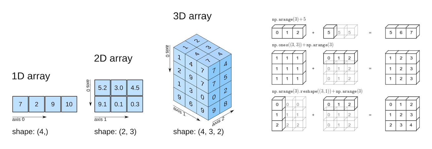
• Tensor
  • 다차원 배열 구조
    • 넘파이와 유사
  • 데이터의 배열로 scalar, vector, matrix 모두를 아우르는 개념
  • 모든 딥러닝 연산의 기본 단위
  • 모델 입출력 구조 이해를 위해 필요
    • 입력 텐서 모양 정확히 알아야 층 설계에 도움이 됨
  • Tensor의 분류
    
    • scalar: 숫자 하나(차원X)
    • vector: 1차원
    • matrix: 2차원
    • tensor: 3차원 이상
      • 이미지, 텍스트(문장) → 3차원 텐서
• 자료형
  • 다양한 타입의 tensor를 지원

PyTorch 타입 이름	실제 자료형(dtype)	설명
HalfTensor	torch.float16	16비트 실수형
FloatTensor	torch.float32	32비트 실수형
DoubleTensor	torch.float64	64비트 실수형
IntTensor	torch.int32	32비트 정수형
LongTensor	torch.int64	64비트 정수형
ShortTensor	torch.int16	16비트 정수형
ByteTensor	torch.uint8	8비트 부호 없는 정수

• Pytorch와 Numpy 간 높은 호환성
  • PyTorch의 Tensor와 Numpy의 ndarray는 유사한 형태를 가지고 있고 PyTorch의 경우 GPU를 사용한 연산이 가능하기 때문에 Numpy로 작업 시 연산 부분을 PyTorch로 대체해서 처리 속도를 끌어 올릴 수 있음(더 알아보기) → 따라서 형태 변경하는 부분을 알아두면 좋음!
    • torch.from_numpy(arr)
    • Tensor.numpy()

Tensor의 연산

• 요소별 연산 가능
  == 관계 연산이 가능하다
  == 불리언 인덱싱이 가능하다

t1 = torch.FloatTensor([[1, 2],
                        [3, 4]])
t2 = torch.FloatTensor([[2, 2],
                        [3, 3]])

# 산술 연산
print("t1+t2\n", t1 + t2)
print("t1-t2\n",t1 - t2)
print("t1*t2\n",t1 * t2)
print("t1/t2\n",t1 / t2)

# 관계 연산
print("t1==t2\n",t1 == t2)
print("t1!=t2\n",t1 != t2)
print("t1<t2\n",t1 < t2)
print("t1>t2\n",t1 > t2)

t1+t2
 tensor([[3., 4.],
        [6., 7.]])
t1-t2
 tensor([[-1.,  0.],
        [ 0.,  1.]])
t1*t2
 tensor([[ 2.,  4.],
        [ 9., 12.]])
t1/t2
 tensor([[0.5000, 1.0000],
        [1.0000, 1.3333]])
t1==t2
 tensor([[False,  True],
        [ True, False]])
t1!=t2
 tensor([[ True, False],
        [False,  True]])
t1<t2
 tensor([[ True, False],
        [False, False]])
t1>t2
 tensor([[False, False],
        [False,  True]])

인플레이스(inplace) 연산

• 연산 후 결과 기존 텐서에 저장
• 기존의 텐서를 변경하여 값을 덮어씌우는 연산을 의미, 원본에 연산을 적용
  • 텐서의 인플레이스 연산은 원본 텐서의 값을 변경하며, 메모리를 절약할 수 있는 장점이 있음
  • 넘파이(In Python)에서 인플레이스(불변객체를 수정하는 것)는 배열의 요소를 수정하거나 변경하는 작업을 의미
    • 인플레이스 작업은 배열의 메모리를 최대한 활용하기 때문에 성능적으로 이점이 있음
• 연산 함수 이름 끝에 _(Underscore, Underbar, Understrike, Underline)가 붙으면 인플레이스 연산에 해당
• 인플레이스 연산은 다음과 같이 _가 연산자 뒤에 붙는 메서드를 사용하여 수행할 수 있음: add_, sub_, mul_, div_, pow_, sqrt_, round_, floor_, ceil_, clamp_, fill_
  • cf. 넘파이에서는 다음과 같은 인플레이스 연산 지원:
    • ndarray.fill(value): 배열의 모든 요소를 지정된 값으로 채웁니다.
    • ndarray.put(indices, values, mode='raise'): 배열에서 지정된 인덱스 위치에 값을 할당합니다.
    • ndarray.clip(min=None, max=None, out=None): 배열의 요소 값을 지정된 최솟값과 최댓값으로 제한합니다.
    • ndarray.sort(axis=-1, kind='quicksort', order=None): 배열의 요소를 정렬합니다.

t1 = torch.FloatTensor([[1, 2],
                        [3, 4]])
t2 = torch.FloatTensor([[2, 2],
                        [3, 3]])

# 덧셈
print("연산자 사용")
print(t1+t2)
print("\n함수 호출 방식")
print(torch.add(t1,t2)) # 함수 호출 방식
print("\n메서드 호출 방식: 인플레이스 연산 X")
print(t1.add(t2)) # 메서드 호출 방식: 인플레이스 연산 X
print('t1:\n', t1)
print("\n메서드 호출 방식: 인플레이스 연산 O")
print(t1.add_(t2)) # 메서드 호출 방식: 인플레이스 연산 O
print('t1:\n',t1)

연산자 사용
tensor([[3., 4.],
        [6., 7.]])

함수 호출 방식
tensor([[3., 4.],
        [6., 7.]])

메서드 호출 방식: 인플레이스 연산 X
tensor([[3., 4.],
        [6., 7.]])
t1:
 tensor([[1., 2.],
        [3., 4.]])

메서드 호출 방식: 인플레이스 연산 O
tensor([[3., 4.],
        [6., 7.]])
t1:
 tensor([[3., 4.],
        [6., 7.]])

# 뺄셈
print("연산자 사용")
print(t1-t2)
print("\n함수 호출 방식")
print(torch.sub(t1,t2)) # 함수 호출 방식
print("\n메서드 호출 방식: 인플레이스 연산 X")
print(t1.sub(t2)) # 메서드 호출 방식: 인플레이스 연산 X
print('t1:\n',t1)
print("\n메서드 호출 방식: 인플레이스 연산 O")
print(t1.sub_(t2)) # 메서드 호출 방식: 인플레이스 연산 O
print('t1:\n',t1)

연산자 사용
tensor([[1., 2.],
        [3., 4.]])

함수 호출 방식
tensor([[1., 2.],
        [3., 4.]])

메서드 호출 방식: 인플레이스 연산 X
tensor([[1., 2.],
        [3., 4.]])
t1:
 tensor([[3., 4.],
        [6., 7.]])

메서드 호출 방식: 인플레이스 연산 O
tensor([[1., 2.],
        [3., 4.]])
t1:
 tensor([[1., 2.],
        [3., 4.]])

행렬곱(the matrix product of two tensors)

• 딥려닝 연산에서 많이 사용되는 연산 중 하나
• 신경망 학습과 추론 과정에서 입력 데이터(X)와 가중치(W)를 연산할 때 사용된다!
• 연산자: @, 함수: torch.matmul, 메서드: Tensor.mm

# 덧셈 -> add
# 뺄셈 -> sub
# 곱셈 -> mul
# 나눗셈 -> div
# 행렬곱 -> mm

t1 = torch.FloatTensor([[1, 2],
                        [3, 4]])
t2 = torch.FloatTensor([[2, 2],
                        [3, 3]])
print(t1)
print(t2)
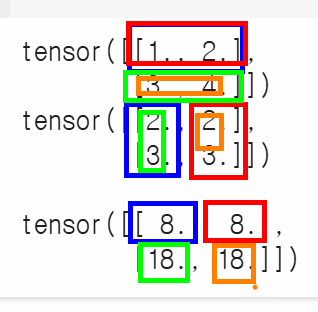
print("\n\n행렬곱:\n", torch.matmul(t1,t2))
# t1 1행 * t2 1열  ->  (1 × 2) + (2 × 3)= 8
# t1 1행 * t2 2열 -> (1 × 2) + (2 × 3) = 8
# t1 2행 * t2 1열 -> (3 × 2) + (4 × 3) = 18
# t1 2행 * t2 2열 -> (3 × 2) + (4 × 3)= 18

tensor([[1., 2.],
        [3., 4.]])
tensor([[2., 2.],
        [3., 3.]])


행렬곱:
 tensor([[ 8.,  8.],
        [18., 18.]])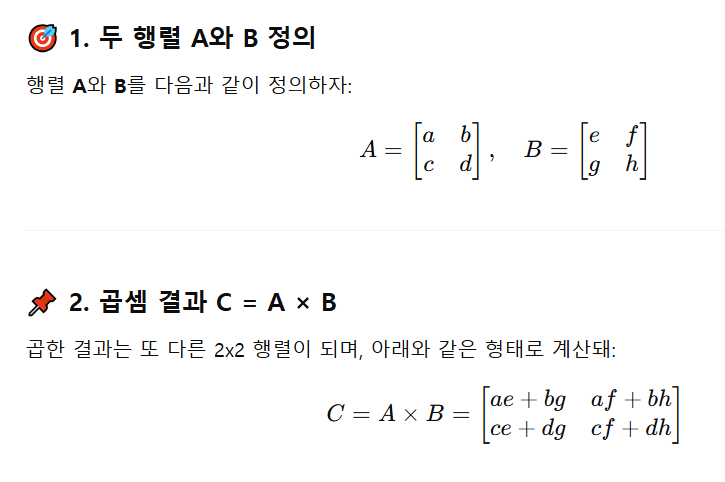

in-place operation

• 객체의 메모리 주소를 변경하지 않고, 기존 객체의 값을 직접 수정하는 연산
• 즉, 새로운 객체를 생성하지 않고 원래 객체 자체를 변경하여 메모리 사용 효율을 높이는 방법
• 인플레이스 연산의 예시:
  • +=, -=, *=, /=, %=와 같은 복합 할당 연산자
    • 변수 자체의 값을 변경
    • 예를 들어, x += 1은 x = x + 1과 동일하지만, x의 메모리 주소를 변경하지 않고 값을 증가시킵니다.
  • list.append(), list.extend(), list.sort()와 같은 리스트 메서드
    • 리스트 객체의 요소를 직접 추가하거나 정렬하여 리스트 자체를 변경
  • pandas 라이브러리의 inplace=True 옵션
    • 일부 pandas 메서드 (예: df.drop(), df.fillna(), df.sort_values())는 inplace=True 옵션을 사용하여 원본 데이터프레임을 직접 수정할 수 있음
• 장점
  • 메모리 효율성
    • 새로운 객체를 생성하지 않으므로 메모리 사용량이 줄어듭니다.
    • 특히 큰 데이터셋을 다룰 때 유용합니다.
  • 성능 향상
    • 객체 생성이 필요 없으므로 연산 속도가 빨라질 수 있습니다.
• 주의사항
  • 예상치 못한 동작
    • inplace=True 옵션을 사용할 때 원본 데이터가 변경될 수 있으므로 주의해야 합니다.
    • 특히 여러 곳에서 동일한 객체를 참조하고 있을 때, 예상치 못한 부작용이 발생할 수 있습니다.
  • 디버깅 어려움
    • 인플레이스 연산은 원본 객체를 변경하므로 디버깅이 어려워질 수 있습니다.
  • 함수형 프로그래밍 지향
    • 파이썬은 함수형 프로그래밍을 지향하며, 인플레이스 연산은 함수형 프로그래밍의 불변성 원칙과 상충될 수 있습니다.
• 인플레이스 연산 사용 시 권장 사항
  • 원본 데이터 복사
    • 인플레이스 연산을 사용하기 전에 필요한 경우 원본 데이터를 복사하여 안전하게 사용해야 합니다.
    • 예를 들어, df_copy = df.copy()와 같이 원본 데이터프레임을 복사하여 사용하면 원본 데이터 변경을 방지할 수 있습니다.
  • 명시적인 코드 작성
    • inplace=True 옵션을 사용할 때는 주석 등을 통해 명시적으로 원본 데이터가 변경됨을 표시하여 다른 개발자들이 코드를 이해하기 쉽도록 해야 합니다.
• 요약:
  • 인플레이스 연산은 메모리 효율성과 성능 향상에 도움이 되지만, 예상치 못한 동작을 유발할 수 있으므로 주의해서 사용해야 합니다.
  • 특히 큰 데이터셋을 다루거나 여러 곳에서 동일한 객체를 참조할 때 더욱 주의해야 합니다.
  • 필요에 따라 원본 데이터를 복사하거나 명시적인 주석을 사용하여 안전하게 인플레이스 연산을 활용하는 것이 좋습니다.

결과값이 다차원인 텐서를 저차원 텐서로 변경하는 방법

t1 = torch.FloatTensor([[1, 2],
                        [3, 4]])
                        
t1.sum() # 출력: tensor(10.)

t1.mean() # 출력: tensor(2.5000)

# 행방향 연산: 열 내에 있는 데이터들을 모두 더함
t1.sum(dim=0) # 출력: tensor([4., 6.])

# 열방향 연산
t1.sum(dim=1)

# dim=-1
t1.sum(dim=-1) # 출력: tensor([3., 7.])
# 가장 마지막 인덱스를 가지는 데이터들의 연산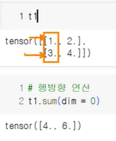

브로드캐스트 연산

• 파이토치에서 차원이 다른 텐서들끼리 연산할 때 자동으로 크기를 맞춰주는 기능
• 선형모델 y=WX+b에서 행렬곱으로 WX 구한 뒤 +b를 계산할 때 많이 사용되는 연산

1. 텐서와 스칼라 연산
   
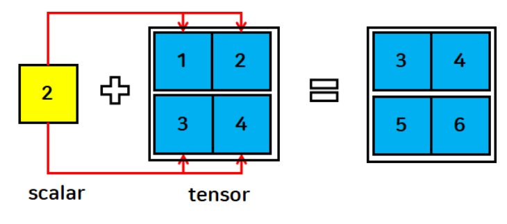
   • 스칼라를 각 텐서에 연산(큰 데이터에 합쳐짐)

t1 = torch.FloatTensor([[1, 2],
                        [3, 4]])
s = 2

print(t1+s)

tensor([[3., 4.],
        [5., 6.]])

2. 텐서와 벡터의 연산
   
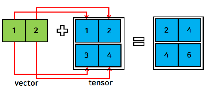
   • 각 행에 동일한 인덱스 벡터를 연산
   • 무조건 브로드캐스팅이 되는 건 아님
     • 브로드캐스트 규칙 위반(shape 불일치) 시 연산 불가
       

v = torch.FloatTensor([1,2])

print(t1+v)

tensor([[2., 4.],
        [4., 6.]])

3. 텐서와 텐서의 연산
   

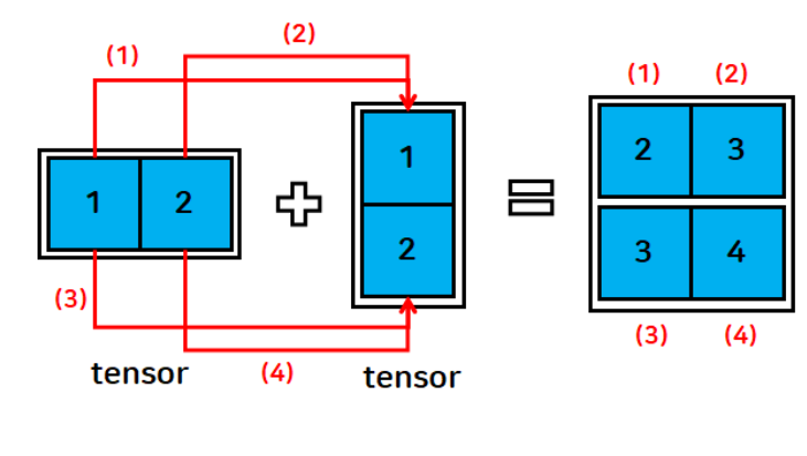
t1 = torch.FloatTensor([[1, 2]])
t2 = torch.FloatTensor([[1], [2]])

print(t1)
print(t1.shape)
print(t2)
print(t2.shape)
print(t1+t2)

tensor([[1., 2.]])
torch.Size([1, 2])
tensor([[1.],
        [2.]])
torch.Size([2, 1])
tensor([[2., 3.],
        [3., 4.]])

브로드캐스트 규칙

• shape 비교를 할 때 뒤에서부터 차례로 비교하며 조건을 확인
  1. 두 개의 차원이 같으면 → 연산 가능
  2. 한 쪽의 차원이 1이면 → 자동으로 확장하여 연산
  3. 두 개의 차원이 다르고 둘 중 하나가 1도 아니면 → 브로드캐스트 불가능(규칙 위반)
• 예시
  • A, B 텐서의 shape 결과가 아래와 같을 때 두 텐서의 더하기하기 연산이 가능한가?
    • A: (4, 3, 2)
    • B: (1, 2)
  • ANSWER: 네, 가능합니다!
    • 맨 뒤부터 비교
      • 2와 2
      • 3과 1
      • 4와 (unsqueezed 1)
    • B가 (1, 2) → (1, 1, 2) → (4, 3, 2)로 자동 확장됨

Tensor 활용 가능한 다양한 함수

view 함수

• 텐서를 원하는 크기로 변경
  • reshape와 동일한 역할
  • reshape보다 빠르고(연속성이 보장되어 있기 때문) 가벼움 → 메모리의 연속이 보장되어 있거나 모델 최적화를 해야 할 경우 사용
• 변환 전, 변환 후 텐서 내의 데이터 개수는 동일해야 함

t1 = torch.FloatTensor([[1, 2], [3, 4], [5, 6], [7, 8]])

t1.view(2,4)

# -1: 요소의 개수에 맞게 값을 자동으로 설정
t1.view(2,-1)
t1.view(2,2,-1)

t3 = t1.view(2,2,-1)
print(t3, t3.shape, sep="\n")

tensor([[[1., 2.],
         [3., 4.]],

        [[5., 6.],
         [7., 8.]]])
torch.Size([2, 2, 2])

# reshape도 사용이 가능하다!
t1.reshape(2,2,-1)

tensor([[[1., 2.],
         [3., 4.]],

        [[5., 6.],
         [7., 8.]]]

view 함수와 reshape 함수의 차이점

• reshape는 언제나 사용 가능
• view 함수는 순차적으로 주소가 할당된 텐서(contiguous tensor)에서만 동작
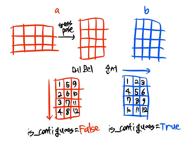
  • 전치행렬을 할 경우 행과 열이 바뀌므로 주소가 순차적으로 할당되지 않음 → view 함수를 사용할 수 없음 → reshape를 사용하면 됨!
    • 전치행렬은 행과 열이 바뀌므로 주소가 순차적으로 할당되지 않음
      
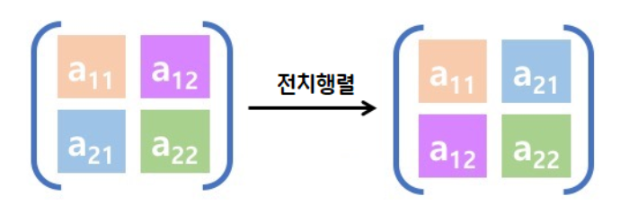
    • 어제 randperm 이용해 숫자 섞은 행렬도 동일한 이유로 view 함수를 쓸 수 없음

view 함수 더 알아보기

• torch.view 함수와 torch.reshape 함수의 원리는 Numpy의 reshape 함수를 기반으로 하고 있음
• torch.view와 torch.reshape의 가장 큰 차이는 contiguous 속성을 만족하지 않는 텐서에 적용이 가능하느냐 여부
• view는 contiguous 속성이 만족되지 않는 경우 일부 사용이 제한됨
• 따라서, 차원 변환을 적용하려는 텐서의 상태에 대하여 정확하게 파악하기가 모호한 경우에는 view 대신 reshape를 사용하는 것을 권장
  • 공식 문서

import torch

x = torch.arange(12)

x # tensor([ 0,  1,  2,  3,  4,  5,  6,  7,  8,  9, 10, 11])

x.reshape(3, 4)
'''
tensor([[ 0,  1,  2,  3],
        [ 4,  5,  6,  7],
        [ 8,  9, 10, 11]])'''

x.view(2, 6)
'''
tensor([[ 0,  1,  2,  3,  4,  5],
        [ 6,  7,  8,  9, 10, 11]])'''

x.reshape(2, 3, -1) # (2, 3, 2) 차원으로 자동 지정
'''
tensor([[[ 0,  1],
         [ 2,  3],
         [ 4,  5]],

        [[ 6,  7],
         [ 8,  9],
         [10, 11]]])'''

x.view(2, 2, -1) # (2, 2, 3) 차원으로 자동 지정
'''
tensor([[[ 0,  1,  2],
         [ 3,  4,  5]],

        [[ 6,  7,  8],
         [ 9, 10, 11]]])'''

x.reshape(2, -1, -1) # RuntimeError: only one dimension can be inferred

x.view(5, -1) # RuntimeError: shape '[5, -1]' is invalid for input of size 12

y = torch.ones(3, 4)

y.transpose_(0, 1)

y.is_contiguous() # False

y.reshape(3, 2, 2) # 실행 가능

y.view(3, 2, 2) # 실행 불가
# RuntimeError: view size is not compatible with input tensor's size and stride (at least one dimension spans across two contiguous subspaces). Use .reshape(...) instead.

• reshape()와 비교:

  • view()는 메모리 공유, reshape()는 메모리 복사 (새로운 메모리 할당)
  • view()는 연속적인 메모리 공간에서만 사용 가능, reshape()는 연속적이지 않아도 동작
  • 메모리 공유로 인한 성능상의 이점, 메모리 복사로 인한 안전성

• 참고:

  • torch.reshape() 함수는 view()와 유사하게 동작하지만, 텐서가 연속적인 메모리 공간에 저장되어 있지 않아도 사용할 수 있습니다. view()가 불가능한 경우, reshape()는 자동으로 새로운 메모리를 할당하여 텐서의 형태를 변경합니다.
  • torch.transpose()는 두 차원의 위치를 변경하는 연산으로, 메모리 구조는 유지하면서 차원만 바꿉니다. view()처럼 메모리를 공유하지만, 연속적인 메모리 구조를 보장하지 않을 수 있습니다.
  • torch.permute()는 여러 차원의 순서를 변경하는 연산입니다.

torch의 contiguous에 대해

• contiguous: 파이토치에서 메모리 내에서의 자료형 저장 상태 중 하나

import torch

a = torch.randn(3, 4)

a.transpose_(0, 1)

b = torch.randn(4, 3)

# 두 tensor는 모두 (4, 3) shape
print(a)
'''
tensor([[-0.7290,  0.7509,  1.1666],
        [-0.9321, -0.4360, -0.2715],
        [ 0.1232, -0.6812, -0.0358],
        [ 1.1923, -0.8931, -0.1995]])'''

print(b)
'''
tensor([[-0.1630,  0.1704,  1.8583],
        [-0.1231, -1.5241,  0.2243],
        [-1.3705,  1.2717, -0.6051],
        [ 0.0412,  1.3312, -1.2066]])'''

# a 텐서 메모리 주소 예시
for i in range(4):
    for j in range(3):
        print(a[i][j].data_ptr())
'''
94418119497152
94418119497168
94418119497184
94418119497156
94418119497172
94418119497188
94418119497160
94418119497176
94418119497192
94418119497164
94418119497180
94418119497196'''

# b 텐서 메모리 주소 예시
for i in range(4):
    for j in range(3):
        print(b[i][j].data_ptr())
'''
94418119613696
94418119613700
94418119613704
94418119613708
94418119613712
94418119613716
94418119613720
94418119613724
94418119613728
94418119613732
94418119613736
94418119613740'''

• 각 데이터의 타입인 torch.float32 자료형은 4바이트이므로, 메모리 1칸 당 주소 값이 4씩 증가함
  • 하지만 위 예제를 자세히 보면 b는 한 줄에 4씩 값이 증가하고 있지만, a는 그렇지 않은 상황임을 알 수 있음

• b는 axis = 0인 오른쪽 방향으로 자료가 순서대로 저장됨에 비해, a는 transpose 연산을 거치며 axis = 1인 아래 방향으로 자료가 저장됨
  • b처럼 axis 순서대로 자료가 저장된 상태를 contiguous = True 상태라고 부르며, a 같이 자료 저장 순서가 원래 방향과 어긋난 경우를 contiguous = False 상태라고 함
• 각 텐서에 stride() 메서드를 호출하여 데이터의 저장 방향을 조회할 수 있음
• is_contiguous() 메서드로 contiguous = True 여부도 쉽게 파악할 수 있음

a.stride() # (1, 4)
b.stride() # (3, 1)

a.is_contiguous() # False
b.is_contiguous() # True

• a.stride() 결과가 (1, 4)라는 것은 a[0][0] -> a[1][0]으로 증가할 때는 자료 1개 만큼의 메모리 주소가 이동되고, a[0][0] -> a[0][1]로 증가할 때는 자료 4개 만큼의 메모리 주소가 바뀐다는 의미
• 텐서의 shape을 조작하는 과정에서 메모리 저장 상태가 변경되는 경우가 존재
  • 주로 narrow(), view(), expand(), transpose() 등 메소드를 사용하는 경우 이 상태가 깨지는 것으로 알려져 있음
• contiguous 여부가 바뀌는 경우, contiguous() 상태의 여부를 체크하지 않더라도 텐서를 다루는데 문제가 없는 경우가 많지만 RuntimeError: input is not contiguous의 오류가 발생하는 경우에는 input tensor를 contiguous = True인 상태로 변경해주어야 할 수 있음
  • 이럴 때에는 아래 예시 코드처럼 contiguous() 메소드를 텐서에 적용하여 contiguous 여부가 True인 상태로 메모리 상 저장 구조를 바꿔줄 수 있음

a.is_contiguous() # False

# 텐서를 contiguous = True 상태로 변경
a = a.contiguous()

a.is_contiguous() # True

squeeze 함수

• 차원의 크기가 1인 차원을 없애주는 기능
• 원하는 차원의 인덱스를 지정하여 수행 가능

t1 = torch.FloatTensor([[[1], [3]]])

print(t1)
# squeeze 함수는 크기가 1인 차원만 제거
print(t1.squeeze(), t1.squeeze().shape, sep="\n")
# 속성 제한 없이 단순하게 사용하면 차원의 크기가 1인 데이터가 모두 사라짐

# 모델에 단일 입력만 넣고 싶을 때
# 이미지 데이터들이 있을 때 단일 이미지로 만들어 보기 쉽게 출력하고 싶을 때
# 모델에 단일 입력만 넣어서 첫 차원을 배제시켜 줄 때(원하는 차원을 제거할 때)

# 첫 번째 차원만 제거하고 싶을 떼
print(t1.squeeze(dim=0), t1.squeeze(dim=0).shape, sep="\n")

# 두 번째 차원을 제거할 수 있나요?
print(t1.squeeze(dim=1), t1.squeeze(dim=1).shape, sep="\n")

# 해당하는 차원의 크기가 1이 아닐 경우 그대로 유지

tensor([[[1.],
         [3.]]])
tensor([1., 3.])
torch.Size([2])
tensor([[1.],
        [3.]])
torch.Size([2, 1])
tensor([[[1.],
         [3.]]])
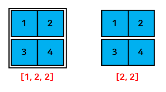
torch.Size([1, 2, 1])

unsqueeze 함수

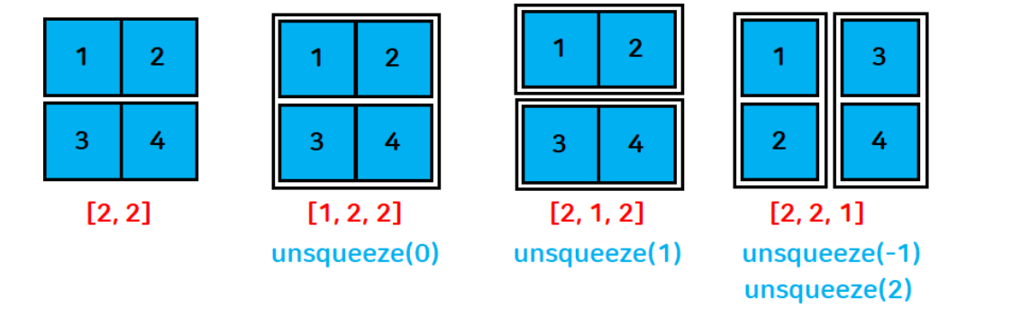
• 현재 차원에서 차원의 크기가 1인 차원을 삽입

t1 = torch.FloatTensor([[1, 2], [3, 4]])
print(t1, t1.shape, sep="\n")

# 0차원(맨 앞)에 크기가 1인 차원을 삽입
print(t1.unsqueeze(dim=0), t1.unsqueeze(dim=0).shape, sep="\n")

# 1차원에 크기가 1인 차원을 삽입
print(t1.unsqueeze(dim=1), t1.unsqueeze(dim=1).shape, sep="\n")

# 2차원에 크기가 1인 차원을 삽입
print(t1.unsqueeze(dim=2), t1.unsqueeze(dim=2).shape, sep="\n")

# dim = -1
print(t1.unsqueeze(dim=-1), t1.unsqueeze(dim=-1).shape, sep="\n")

tensor([[1., 2.],
        [3., 4.]])
torch.Size([2, 2])
tensor([[[1., 2.],
         [3., 4.]]])
torch.Size([1, 2, 2])
tensor([[[1., 2.]],

        [[3., 4.]]])
torch.Size([2, 1, 2])
tensor([[[1.],
         [2.]],

        [[3.],
         [4.]]])
torch.Size([2, 2, 1])
tensor([[[1.],
         [2.]],

        [[3.],
         [4.]]])
torch.Size([2, 2, 1])

• reshape 함수를 사용하여 차원 추가, 제거 가능

t1 = torch.FloatTensor([[1, 2], [3, 4]])
print(t1.reshape(2,2,1))

# reshape에서 -1을 사용하면 기존 텐서의 크기에 맞춰 할당
print(t1.reshape(2,-1,1), t1.reshape(2,-1,1).shape, sep="\n")

tensor([[[1.],
         [2.]],

        [[3.],
         [4.]]])
tensor([[[1.],
         [2.]],

        [[3.],
         [4.]]])
torch.Size([2, 2, 1])

인덱싱

• indexing: 원하는 tensor에서 요소를 검색 → 추출
• slicing: 범위를 주어 원하는 tensor 요소 검색 → 추출
  • 텐서명[시작 인덱스:끝 인덱스+1]
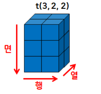
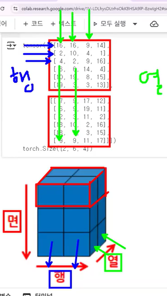
• 3차원 데이터: [면, 행, 열]
  

cf. 넘파이 ndarray의 데이터 세트 선택하기: 인덱싱(indexing)

• 넘파이에서 ndarray 내의 일부 데이터 세트나 특정 데이터만을 선택할 수 있음
  1. 특정한 데이터만 추출
     • 원하는 위치의 인덱스 값을 지정하면 해당 위치의 데이터가 반환됨
  2. 슬라이싱(Slicing)
     • 연속된 인덱스상의 ndarray를 추출하는 방식
     • : 기호 사이에 시작 인덱스와 종료 인덱스를 표시하면 시작 인덱스에서 (종료 인덱스 - 1) 위치에 있는 데이터의 ndarray를 반환
  3. 팬시 인덱싱(Fancy Indexing)
     • 일정한 인덱싱 집합을 리스트 또는 ndarray 형태로 지정해 해당 위치에 있는 데이터의 ndarray를 반환
  4. 불린 인덱싱(Boolean Indexing)
     • 특정 조건에 해당하는지 여부인 True/False 값 인덱싱 집합을 기반으로 True에 해당하는 인덱스 위치에 있는 데이터의 ndarray 반환

torch.randint(1, 20, size=(3,2,2))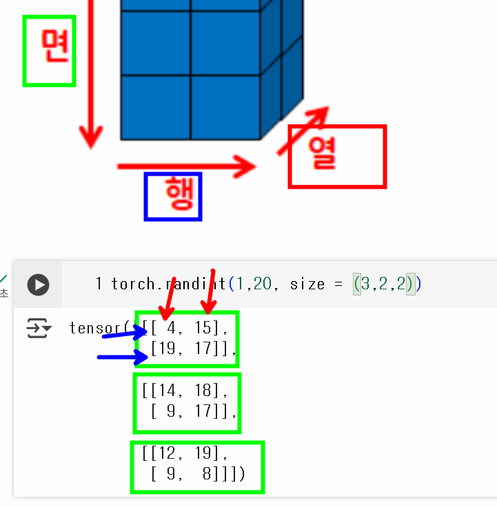

# 1~50까지 1씩 증가하는 2차원 배열(5행 10열)
t = torch.arange(1,51).reshape(5,10) # .reshape(5,-1)도 가능

# 13 인덱싱하기
print(t[1,2]) # print(t[1][2])도 가능

# 15,16,17 슬라이싱
print(t[1,4:7]) # print(t[1][4:7])도 가능
# 텐서명[면, 행, 렬]

# 전체 행의 0열 출력
t[:,0]

# 3행의 전체 열
t[3,:]

# 전체 행의 0~2열
t[:,:3]

# 35만 가져오기
t[3,4]

# 22, 33 두 개 출력
t[[2,3],[1,2]]
# 22 → 2행 1열
# 33 → 3행 2열

# 23, 32, 35
t[[2,3,3],[2,1,4]]

tensor(13)
tensor([15, 16, 17])
tensor([ 1, 11, 21, 31, 41])
tensor([31, 32, 33, 34, 35, 36, 37, 38, 39, 40])
tensor([[ 1,  2,  3],
        [11, 12, 13],
        [21, 22, 23],
        [31, 32, 33],
        [41, 42, 43]])
tensor(35)
tensor([22, 33])
tensor([23, 32, 35])

• 3차원 텐서의 인덱싱, 슬라이싱
  • 이미지에서 내가 원하는 채널별 슬라이싱
  • 텍스트에서 특정 단어만 추출 등

t3 = torch.randint(1, 20, size=(3,2,2))
# (면, 행, 열)
print(t3)

# 첫 번째 면 추출
print(t3[0])

# 마지막 면 추출
print(t3[-1])

# 첫 번째 행 추출
# 면, 행, 열 데이터
t3[:,0] # 또는 t3[:,0,:]

# 첫 번째 열 추출
t3[:,:,0]

t3[1,1,:] # 필요한 것만 핀포인트로 뽑아옴
t3[1:2,1:,:] # 현재 차원 상태가 그대로 유지

tensor([[[ 7, 11],
         [18, 15]],

        [[11, 19],
         [ 8,  4]],

        [[ 7,  4],
         [ 7, 16]]])
tensor([[ 7, 11],
        [18, 15]])
tensor([[ 7,  4],
        [ 7, 16]])
tensor([[ 7, 11],
        [11, 19],
        [ 7,  4]])
tensor([[ 7, 18],
        [11,  8],
        [ 7,  7]])
tensor([8, 4])
tensor([[[8, 4]]])

split 함수

• 텐서를 특정 차원에서 원하는 형태로 분리

t = torch.randint(1, 20, size=(2,6,4)) # 2면 6행 4열

# 행을 3개씩 분리
# 총 6행이기 때문에 2개의 행으로 분리됨
t.split(3, dim=1)

# 열을 2개씩 분리
t.split(2, dim=2)

# 3개씩 열로 분리 → 4열이므로 3개와 1개 열의 텐서로 분리
t.split(3, dim=2)

# 면을 1개씩 분리: 2면이므로 1개와 1개로 tensor 분리
t.split(1)
# dim의 default 값은 0 (dim=0)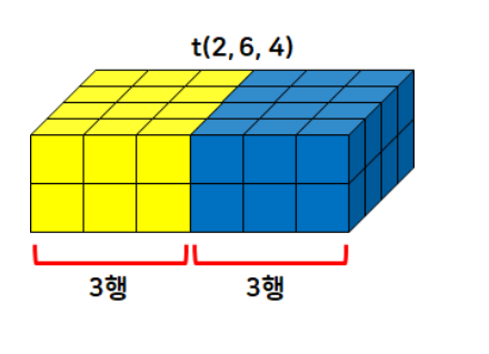

chunk 함수

• 텐서를 특정 타원에 대해 크기와 상관없이 개수만큼 분리

t2 = t.chunk(3, dim=1)
print(t.shape) # 행이 2개씩 나눠진다~
print(t2)

torch.Size([2, 6, 4])
(tensor([[[13,  8,  9,  4],
         [ 3, 12,  4, 14]],

        [[11, 18, 16, 10],
         [ 8, 13,  7, 10]]]), tensor([[[13, 16,  1,  6],
         [ 4,  1, 13, 16]],

        [[19,  5,  9, 11],
         [ 2,  5,  3,  8]]]), tensor([[[19, 10, 18,  9],
         [15, 19,  5, 10]],

        [[ 2,  6,  3,  5],
         [17, 17, 17, 12]]]))

# 열을 2개의 텐서로 분리
t.chunk(2, dim=2)

(tensor([[[13,  8],
          [ 3, 12],
          [13, 16],
          [ 4,  1],
          [19, 10],
          [15, 19]],
 
         [[11, 18],
          [ 8, 13],
          [19,  5],
          [ 2,  5],
          [ 2,  6],
          [17, 17]]]),
 tensor([[[ 9,  4],
          [ 4, 14],
          [ 1,  6],
          [13, 16],
          [18,  9],
          [ 5, 10]],
 
         [[16, 10],
          [ 7, 10],
          [ 9, 11],
          [ 3,  8],
          [ 3,  5],
          [17, 12]]]))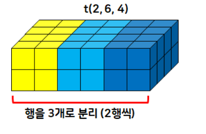

• torch.chunk(input: Tensor, chunks: int, dim: int = 0) → Tuple[Tensor, ...]
  • This function may return fewer than the specified number of chunks!
  • If the tensor size along the given dimension dim is divisible by chunks, all returned chunks will be the same size. If the tensor size along the given dimension dim is not divisible by chunks, all returned chunks will be the same size, except the last one. If such division is not possible, this function may return fewer than the specified number of chunks.

>>> torch.arange(11).chunk(6)
(tensor([0, 1]),
 tensor([2, 3]),
 tensor([4, 5]),
 tensor([6, 7]),
 tensor([8, 9]),
 tensor([10]))
>>> torch.arange(12).chunk(6)
(tensor([0, 1]),
 tensor([2, 3]),
 tensor([4, 5]),
 tensor([6, 7]),
 tensor([8, 9]),
 tensor([10, 11]))
>>> torch.arange(13).chunk(6)
(tensor([0, 1, 2]),
 tensor([3, 4, 5]),
 tensor([6, 7, 8]),
 tensor([ 9, 10, 11]),
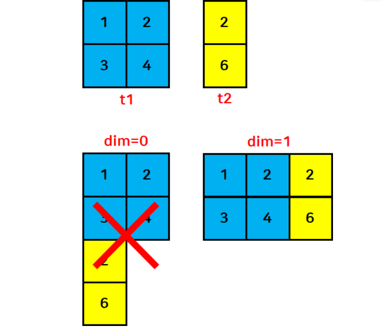
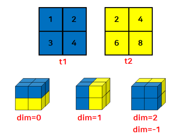
 tensor([12]))

cat 함수

• 2개 이상의 함수를 순서대로 병합하여 하나의 텐서로 만듦
• 2차원 텐서인 경우:
  
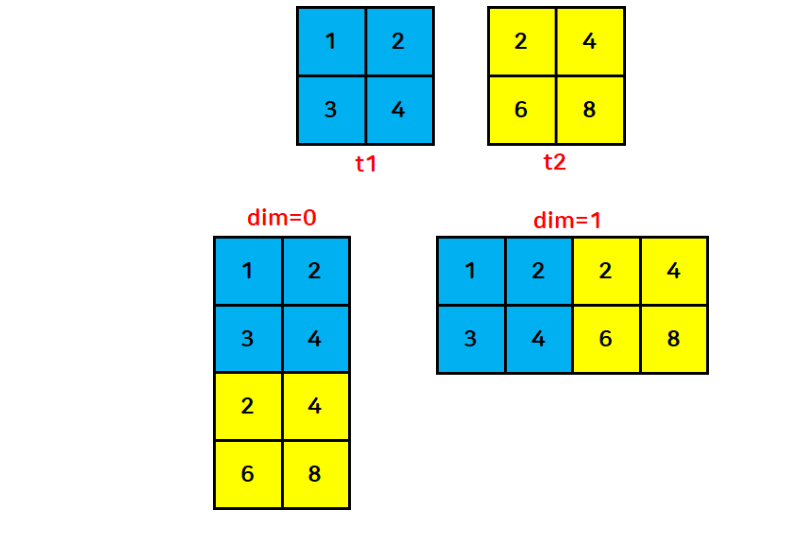
  • dim=0이면 행끼리 → 병합 결과 (4,2)
  • dim=1이면 열끼리 병합 → (2,4)
• 3차원 텐서(2,2,2)인 경우:
  • dim=0이면 면끼리 → (4,2,2)
  • dim=1이면 행끼리 → (2,4,2)
  • dim=2면 열끼리 병합 → (2,2,4)

t1 = torch.FloatTensor([[1, 2], [3, 4]])
t2 = torch.FloatTensor([[2, 4], [6, 8]])

# 행 방향으로 병합
print(torch.cat([t1, t2], dim=0))

# 열 방향으로 병합
print(torch.cat([t1,t2],dim=1))

tensor([[1., 2.],
        [3., 4.],
        [2., 4.],
        [6., 8.]])
tensor([[1., 2., 2., 4.],
        [3., 4., 6., 8.]])

• 병합할 텐서의 차원이 다르면 병합할 수 없다!
  

stack 함수

• 2개 이상의 텐서를 원하는 방향으로 병합
  
• cat 함수와의 차이점
  • 새로운 차원으로 확장하여 병합(차원을 증가시킴)

t1 = torch.FloatTensor([[1, 2], [3, 4]])
t2 = torch.FloatTensor([[2, 4], [6, 8]])

torch.stack([t1, t2], dim=0)

tensor([[[1., 2.],
         [3., 4.]],

        [[2., 4.],
         [6., 8.]]])

index_select 함수

• 불연속적인 인덱스 값을 반환
  

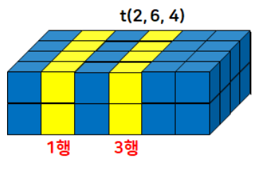
t = torch.randint(1,20,size=(2,6,4))
print(t, t.dtype, sep="\n")
# 자료형: LongTensor

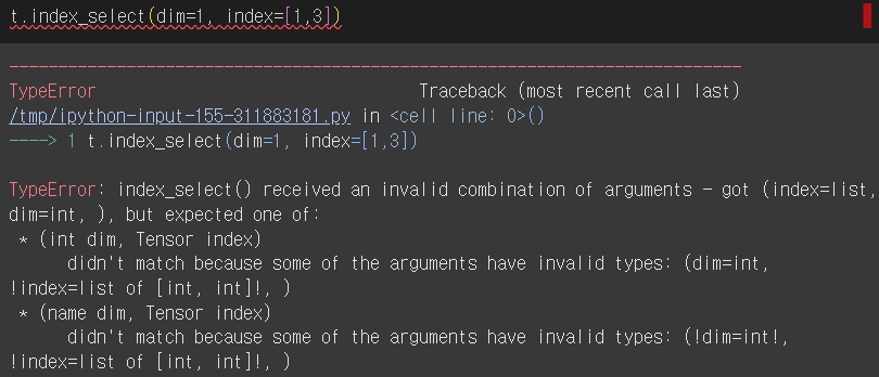
print(t.index_select(dim=1, index=torch.LongTensor([1,3])))
# 인덱스는 반드시 텐서로 넣어줘야 함!
# index (IntTensor or LongTensor)

tensor([[[ 8, 15, 12,  1],
         [ 5, 16, 13, 19],
         [ 3,  2,  1, 12],
         [ 7,  1, 10, 18],
         [10, 11, 11, 11],
         [ 7, 17,  7, 11]],

        [[ 1,  8,  1,  8],
         [14, 18, 18, 11],
         [ 1, 15, 19, 11],
         [16,  4, 19, 15],
         [ 9,  7,  4, 13],
         [12,  6,  1, 16]]])
torch.int64
tensor([[[ 5, 16, 13, 19],
         [ 7,  1, 10, 18]],

        [[14, 18, 18, 11],
         [16,  4, 19, 15]]])

• 인덱스를 IntTensor나 LongTensor로 넣지 않으면 오류 발생
  

면/헹/열 형태와 인덱싱 작성법 잘 이해하기

argmax 함수

• arguments of the maxima
  • a function that returns the index or argument of the maximum value in a set or array
    • the function argument x at which the maximum of f occurs
    • an operation that finds the argument that gives the maximum value from a target function
• Tensor.argmax(dim=None, keepdim=False) → LongTensor 또는 torch.argmax(input) → LongTensor
• 요소들 중에서 가장 큰 값의 인덱스 반환

t = torch.randperm(9).reshape(3,3)
print(t)
print(t.argmax())

# 행끼리 비교했을 때 가장 큰 값을 가지는 인덱스를 추출
print(t.argmax(dim=0))
# 행 방향으로 이동하며 비교

# 열끼리 비교했을 때 가장 큰 값을 가지는 인덱스를 추출
print(t.argmax(dim=1))

tensor([[4, 6, 0],
        [8, 7, 1],
        [2, 5, 3]])
tensor(3)
tensor([1, 1, 2])
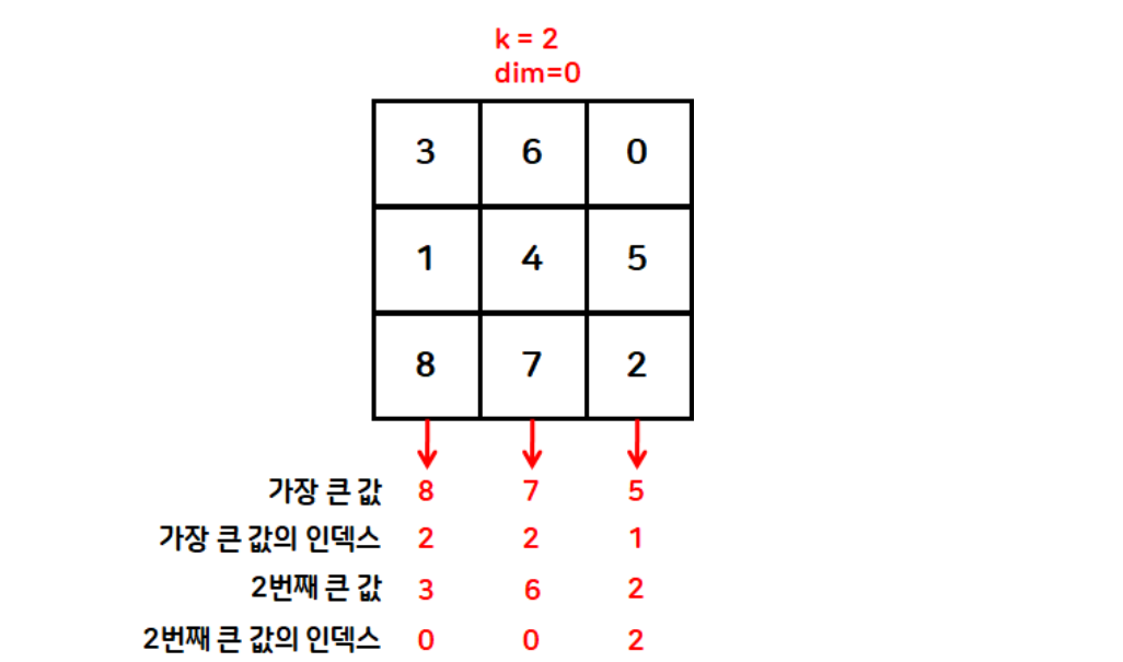
tensor([1, 0, 1])

topk 함수

• 상위 k개의 값과 인덱스를 반환
  

t = torch.randperm(9).reshape(3,3)
print(t)
print(torch.topk(t, k=2, dim=0))

# 오름차순 정렬
torch.topk(t, k=t.size(dim=0), largest=False)

tensor([[6, 0, 5],
        [4, 7, 8],
        [1, 2, 3]])
torch.return_types.topk(
values=tensor([[6, 7, 8],
        [4, 2, 5]]),
indices=tensor([[0, 1, 1],
        [1, 2, 0]]))
torch.return_types.topk(
values=tensor([[0, 5, 6],
        [4, 7, 8],
        [1, 2, 3]]),
indices=tensor([[1, 2, 0],
        [0, 1, 2],
        [0, 1, 2]]))

# 보통 randperm 에 대해 오름차순 정렬 많이 진행함
t = torch.randperm(9)
print(t)
torch.topk(t, k=t.size(dim=0), largest=False)

tensor([2, 1, 6, 5, 0, 8, 7, 3, 4])
torch.return_types.topk(
values=tensor([0, 1, 2, 3, 4, 5, 6, 7, 8]),
indices=tensor([4, 1, 0, 7, 8, 3, 2, 6, 5]))

masked_fill 함수

• 텐서 내의 조건에 맞는 데이터를 특정 값으로 변경

t = torch.randperm(9).reshape(3,3)
print(t)
# 텐서 내의 데이터 중에서 5보다 큰 값을 -1로 변경
print(t.masked_fill(t>5, value=-1))

# 다중 조건 설정 가능
print(t.masked_fill((t>5)|(t==0), value=-1))

tensor([[1, 0, 8],
        [7, 6, 2],
        [5, 3, 4]])
tensor([[ 1,  0, -1],
        [-1, -1,  2],
        [ 5,  3,  4]])
tensor([[ 1,  -1, -1],
        [-1, -1,  2],
        [ 5,  3,  4]])

---

---

하루 돌아보기

👍 잘한 점

• 쉬는 시간 활용해서 오늘 배운 내용 6시 전에 모두 복습 완료
  • 강의 녹화본 올라오면 한 번 더 복습할 예정
• 파이썬 패킹/언패킹 개념 복습
  • 다른 분이 작성한 코드에 등장해서 다시 살펴봄

👎 아쉬웠던 점

• 미니 프로젝트 팀이 정해졌는데 아직 어색해서 적극적으로 소통을 못 했음

🔬 개선점

• 내일 프로젝트 주제 발표되고 나면 좀 더 적극적으로 소통하기