[인공지능사관학교: 자연어분석A반] 학습 내용 보충 - 경사하강법 직접 구현하기
테디노트: PyTorch의 자동미분(AutoGrad)기능과 경사하강법(Gradient Descent) 구현
✅
PyTorch의 자동미분(AutoGrad) 기능을 활용하여 경사하강법 알고리즘 직접 구현하기
✅ 손실(loss) 값과weight,bias변화량 시각화하기
PyTorch로 경사하강법(Gradient Descent) 구현
- 기본 개념은 함수의 기울기(경사)를 구하여 기울기가 낮은 쪽으로 계속 이동시켜서 극값에 이를 때까지 반복시키는 것
- 비용 함수 (Cost Function 혹은 Loss Function)를 최소화하기 위해 반복해서 파라미터를 업데이트
- 더 상세한 설명은:
# 모듈 import
from IPython.display import Image
import matplotlib.pyplot as plt
import numpy as np
import torch
샘플 데이터셋 생성
y = 0.3x + 0.5의 선형회귀 식을 추종하는 샘플 데이터셋을 생성- 경사하강법 알고리즘으로
w=0.3,b=0.5를 추종하는 결과를 도출
def make_linear(w=0.5, b=0.8, size=50, noise=1.0):
    x = np.random.rand(size)
    y = w * x + b
    noise = np.random.uniform(-abs(noise), abs(noise), size=y.shape)
    yy = y + noise
    plt.figure(figsize=(10, 7))
    plt.plot(x, y, color='r', label=f'y = {w}x + {b}', linestyle=':', alpha=0.3)
    plt.scatter(x, yy, color='black', label='data', marker='.')
    plt.legend(fontsize=15)
    plt.show()
    print(f'w: {w}, b: {b}')
    return x, yy

x, y = make_linear(w=0.3, b=0.5, size=100, noise=0.01)

# w: 0.3, b: 0.5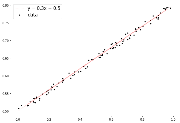
- 샘플 데이터셋인 x와 y를 텐서(Tensor)로 변환(
torch.as_tensor())하고 랜덤한 w, b 생성- torch.rand(1)은 torch.Size([1])을 가지는 normal 분포의 랜덤 텐서를 생성
# 샘플 데이터셋을 텐서(tensor)로 변환
x = torch.as_tensor(x)
y = torch.as_tensor(y)

# random 한 값으로 w, b를 초기화 합니다.
w = torch.rand(1)
b = torch.rand(1)

print(w.shape, b.shape)

# requires_grad = True로 설정된 텐서에 대해서만 미분을 계산합니다.
w.requires_grad = True
b.requires_grad = True

# torch.Size([1]) torch.Size([1])- 가설함수(Hypothesis Function) 정의하고 y_hat과 y의 손실(Loss)를 계산
- 가설함수는 Affine Function을 정의함
- 손실함수는 Mean Squared Error 함수를 사용
# Hypothesis Function 정의
y_hat = w * x + b

# 손실함수 정의
loss = ((y_hat - y)**2).mean()- loss.backward() 호출시 미분 가능한 텐서(Tensor)에 대하여 미분을 계산
# 미분 계산 (Back Propagation)
loss.backward()- w와 b의 미분 값 확인
# 계산된 미분 값 확인
w.grad, b.grad

# 출력: (tensor([-0.6570]), tensor([-1.1999]))
경사하강법 구현
- 최대 500번의 iteration(epoch) 동안 반복하여 w, b의 미분을 업데이트 하면서, 최소의 손실(loss)에 도달하는 w, b를 산출
- learning_rate는 임의의 값으로 초기화, 0.1로 설정
# 하이퍼파라미터(hyper-parameter) 정의

# 최대 반복 횟수 정의
num_epoch = 500

# 학습율 (learning_rate)
learning_rate = 0.1

# loss, w, b 기록하기 위한 list 정의
losses = []
ws = []
bs = []

# random 한 값으로 w, b를 초기화 합니다.
w = torch.rand(1)
b = torch.rand(1)

# 미분 값을 구하기 위하여 requires_grad는 True로 설정
w.requires_grad = True
b.requires_grad = True

for epoch in range(num_epoch):
    # Affine Function
    y_hat = x * w + b

    # 손실(loss) 계산
    loss = ((y_hat - y)**2).mean()

    # 손실이 0.00005보다 작으면 break 합니다.
    if loss < 0.00005:
        break

    # w, b의 미분 값인 grad 확인시 다음 미분 계산 값은 None이 return 됩니다.
    # 이러한 현상을 방지하기 위하여 retain_grad()를 loss.backward() 이전에 호출해 줍니다.
    w.retain_grad()
    b.retain_grad()

    # 미분 계산
    loss.backward()

    # 경사하강법 계산 및 적용
    # w에 learning_rate * (그라디언트 w) 를 차감합니다.
    w = w - learning_rate * w.grad
    # b에 learning_rate * (그라디언트 b) 를 차감합니다.
    b = b - learning_rate * b.grad

    # 계산된 loss, w, b를 저장합니다.
    losses.append(loss.item())
    ws.append(w.item())
    bs.append(b.item())

    if epoch % 5 == 0:
        print("{0:03d} w = {1:.5f}, b = {2:.5f} loss = {3:.5f}".format(epoch, w.item(), b.item(), loss.item()))

print("----" * 15)
print("{0:03d} w = {1:.1f}, b = {2:.1f} loss = {3:.5f}".format(epoch, w.item(), b.item(), loss.item()))
결과 시각화
- loss는 epoch이 늘어남에 따라 감소
- epoch 초기에는 급격히 감소하다가, 점차 완만하게 감소함을 확인 가능
- 이는 초기에는 큰 미분 값이 업데이트 되지만, 점차 계산된 미분 값이 작아지게되고 결국 업데이트가 작게 일어나면서 손실은 완만하게 감소하기 때문
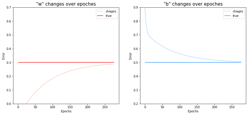
- w, b도 초기값은 0.3, 0.5와 다소 먼 값이 설정되었지만, 점차 정답을 찾아감
# 전체 loss 에 대한 변화량 시각화
plt.figure(figsize=(14, 6))
plt.plot(losses, c='darkviolet', linestyle=':')

plt.title('Losses over epoches', fontsize=15)
plt.xlabel('Epochs')
plt.ylabel('Error')
plt.show()

# w, b에 대한 변화량 시각화
fig, axes = plt.subplots(1, 2)
fig.set_size_inches(14, 6)

axes[0].plot(ws, c='tomato', linestyle=':', label='chages')
axes[0].hlines(y=0.3, xmin=0, xmax=len(ws), color='r', label='true')
axes[0].set_ylim(0, 0.7)
axes[0].set_title('"w" changes over epoches', fontsize=15)
axes[0].set_xlabel('Epochs')
axes[0].set_ylabel('Error')
axes[0].legend()

axes[1].plot(bs, c='dodgerblue', linestyle=':', label='chages')
axes[1].hlines(y=0.5, xmin=0, xmax=len(ws), color='dodgerblue', label='true')
axes[1].set_ylim(0.2, 0.9)
axes[1].set_title('"b" changes over epoches', fontsize=15)
axes[1].set_xlabel('Epochs')
axes[1].set_ylabel('Error')
axes[1].legend()

plt.show()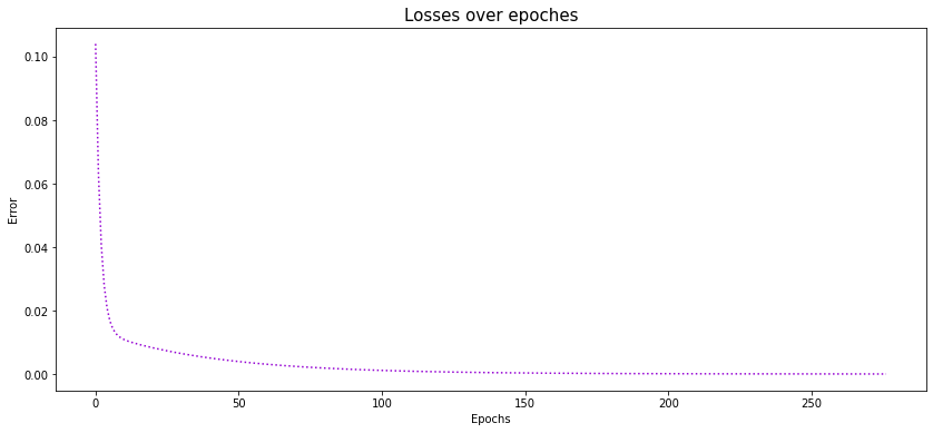

2 B R 0 2 B