머신러닝 특강: 분류 분석

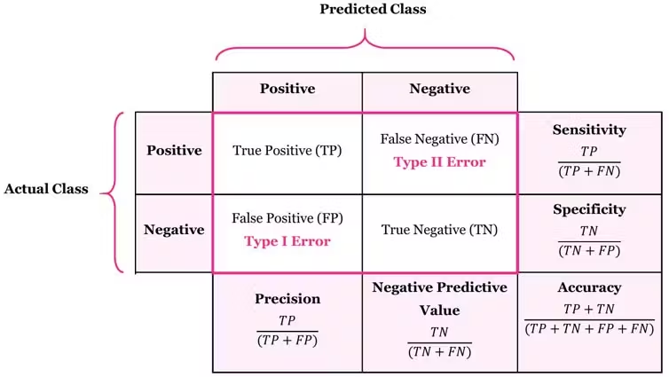
혼동 행렬(Confusion Matrix)
- 모델이 예측한 결과와 실제 결과를 비교하여 만들어진 행렬(테이블)
- 모델의 분류 성능을 한 눈에 알 수 있어서 편리
구분(실제 - 모델 순)
- TP(True Positive)
  - 실제 양성을 양성으로 분류한 경우
- FP(False Positive)
  - 실제 음성을 양성으로 분류한 경우
- TN(True Negative)
  - 실제 음성을 음성으로 분류한 경우
- FN(False Negative)
  - 실제 양성을 음성으로 분류한 경우
분류 모델의 성능 지표
- 정확도(Accuracy)
  - 전체 데이터 셋에서 실제 값을 제대로 맞춘 비율

\text{Accuracy} = \frac{TP + TN}{TP + TN + FP + FN}

정밀도(Precision)
- 모델이 양성으로 분류한 값 중에서 실제 양성의 비율

\text{Precision} = \frac{TP}{TP + FP}

민감도(Sensitivity)
- 실제 값이 양성인 데이터 중에서 양성으로 분류한 비율
- 재현율(Recall)이라고도 함

\text{Sensitivity (Recall)} = \frac{TP}{TP + FN}

F1 Score
- 정밀도와 재현율의 조화 평균

\text{F1 Score} = 2 \times \frac{\text{Precision} \times \text{Recall}}{\text{Precision} + \text{Recall}}

분류 모형

아래 모델들은 분류 문제에 자주 사용되는 모형들입니다.
- 로지스틱 회귀(Logistic Regression)
- K Nearest(K-NN)
- 나이브 베이즈(Naive Bayes)
- 서포트 벡터 머신(Support Vector Machine)
- 랜덤 포레스트(Random Forest)
- 다층 퍼셉트론 (Multi-Layer Perceptron)

로지스틱 회귀 분석 (Logistic Regression)

Logarithms and Logistic Growth

정의

독립 변수의 선형 결합을 이용해서 사건의 발생 가능성(확률)을 예측하는 데 사용되는 모델
타겟 변수가 주로 두 개의 범주(Yes/No)인 경우에 주로 사용
이름에서 나타나는 것처럼 Log를 활용한 계산이 들어감

모델 설명

오즈 (Odds)
- 성공 확률이 실패 확률에 비해 몇 배 더 높은지를 나타냄
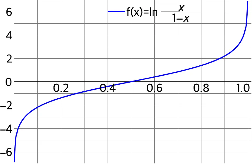
- 도박사들이 주로 쓰는 표기 $\text{Odds} = \frac{P(\text{success})}{P(\text{failure})} = \frac{p}{1-p}$
로짓 (Logit)
- 오즈에 자연로그를 취한 값
- 확률 p에 대해 (−∞,+∞) 범위로 출력값을 조절 $\text{Logit}(p) = \ln(\text{Odds}) = \ln(\frac{p}{1-p})$
로지스틱 함수
- 선형 회귀식의 결과를 0과 1 사이의 확률값으로 변환하는 함수
- 선형 회귀식의 결과는 연속형으로 0과 1 사이 범위를 초과할 수 있어 이를 로짓 변화를 통해 변환
  - 도출 과정은 블로그 참고

P(X) = \frac{1}{1 + e^{-(\beta_0 + \beta_1X_1 + ... + \beta_nX_n)}}

출처 - https://medium.com/@vikrampande783/derivative-of-sigmoid-and-tanh-ffdea6efb464

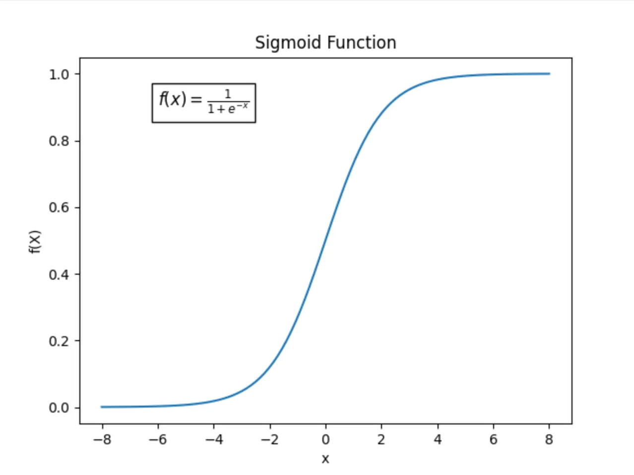
로지스틱 회귀식은 다음과 같이 변형 가능:
$\frac{P}{1-P} = e^{(\beta_0 + \beta_1X_1 + ... + \beta_nX_n)}$
- 선형회귀 값이 0인 경우 → P(X) = 0.5
- 값이 0보다 크면 P(X)가 1에 가까워지고, 0보다 작으면 P(X)가 0에 가까워짐
  - 특정 값(Threshold)을 기준으로 값이 높은 경우 1, 그렇지 않으면 0으로 분류
- X_n의 값이 1만큼 증가하면, 오즈비는 e^beta_n 만큼 증가

다중 클래스 분류

로지스틱 회귀 분석은 이진 분류에 주로 사용되지만, 클래스가 3개 이상인 다중 클래스 분류에도 활용할 수 있음
방법
1. One-Hot encoding을 통해 N개의 클래스를 N 차원의 벡터로 변환
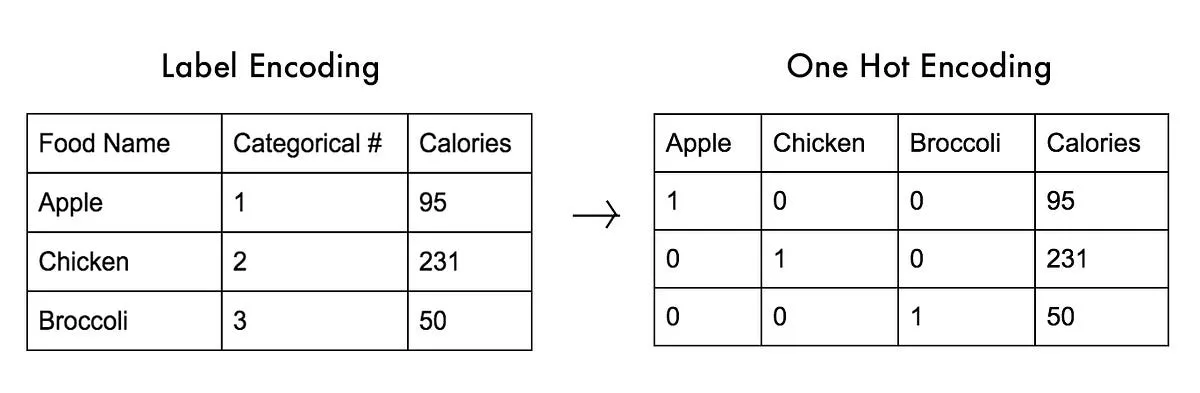
2. 각각의 차원에 대해서 로지스틱 회귀 분석을 수행
3. 이때 각 차원의 예측값은 해당 클래스에 분류될 확률에 해당함
4. 확률이 가장 높게 나온 클래스로 해당 데이터를 분류
  - 이를 Hard Clustering이라고 함!

랜덤 포레스트

정의

여러 개의 의사결정나무(Decision Tree)를 학습시켜 성능을 높이는 앙상블 학습 방법

의사결정나무(Decision Tree)

출처 - https://blog-ko.superb-ai.com/3-minute-algorithm-decision-tree/

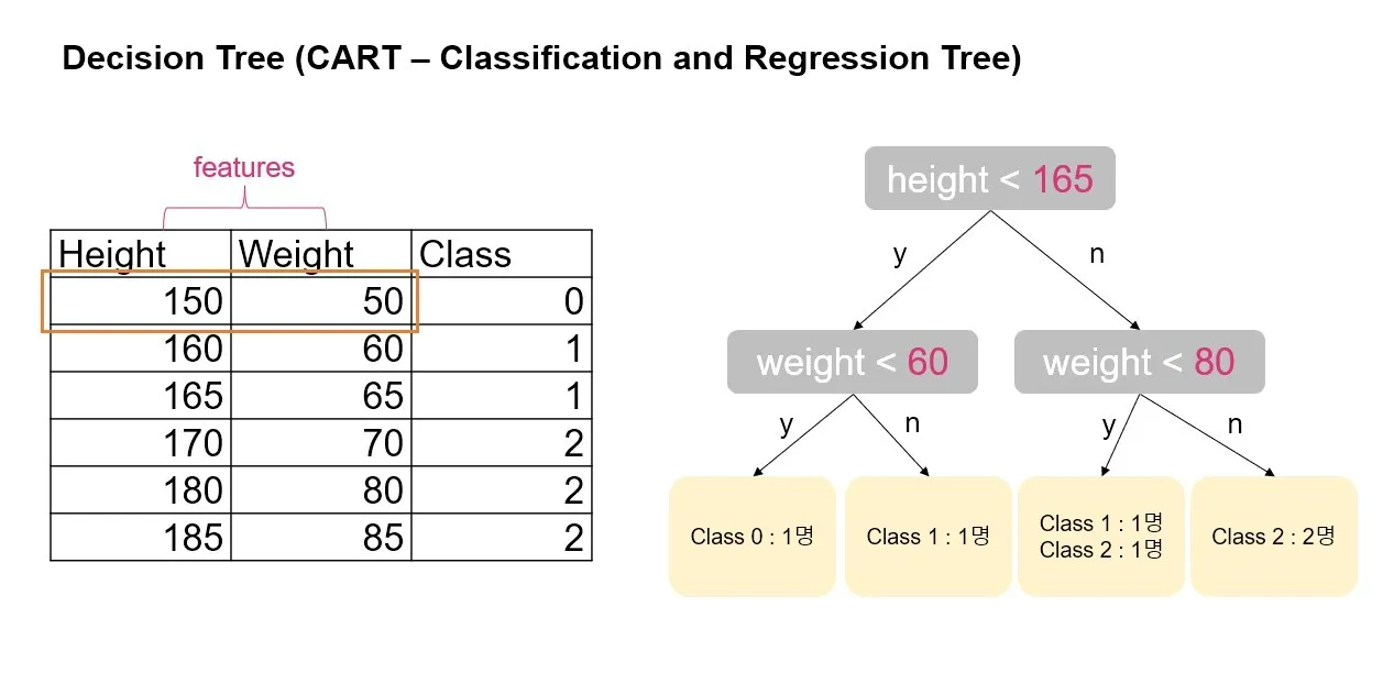
한 번에 하나의 기준으로 데이터를 두 그룹으로 분류해 나감
데이터를 분류할 때는 불순도가 낮아지는 방향으로 분류
- 불순도
  - 한 집단에 각기 다른 클래스의 비중이 비슷하게 있다면 불순도가 높은 상태
  - 불순도가 낮은 방향 → 두 그룹으로 나눴을 때 각각의 그룹은 비슷한 클래스끼리 묶여 있게 됨
스무고개를 생각하면 이해하기 쉬움

분류하고 나서 두 집단 내에 적합하지 않은 샘플이 얼마나 끼어 있냐 정도로 해석할 수 있습니다.
스무고개 질문 게임을 진행할 때
질문을 많이 거칠 수록 정답에 가까워 지는 현상(순도가 높아짐)

앙상블(Ensemble)

하나의 모델을 사용하는 것이 아닌, 여러 개의 모델을 결합하여 모델의 성능을 높이는 방식
예시
- 배깅 (Bagging)
- 부스팅 (Boosting)

랜덤 포레스트(Random Forest)

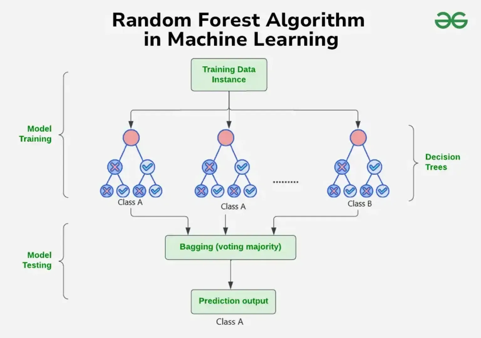
설명
- 여러 개의 의사결정나무를 결합하여 분류 및 예측 모델에 활용하는 모델로 대표적인 앙상블 모델 중 하나
- 각각의 트리를 학습할때마다 Feature의 일부만을 랜덤하게 선택하여 사용
- 분류 모델의 경우, 여러 의사결정나무에서 분류한 결과에서 투표를 통해 최종 결과를 선택
Feature Importance
- 각각의 의사결정나무를 학습할 때 어떤 Feature가 많이 사용되었는지에 따라서 모델 생성에 중요하게 동작한 Feature를 선정할 수 있음

실습

위에서 배운 내용을 바탕으로 분류 모델 예제 코드를 살펴보기
# UIC 데이터 호출을 위한 패키지 설치
!pip install ucimlrepo

import numpy as np
import pandas as pd
import matplotlib.pyplot as plt
import seaborn as sns
import math

from ucimlrepo import fetch_ucirepo

from sklearn.linear_model import LogisticRegression
from sklearn.model_selection import train_test_split, GridSearchCV
from sklearn.preprocessing import StandardScaler, OneHotEncoder
from sklearn.ensemble import RandomForestClassifier
from sklearn.metrics import classification_report, confusion_matrix

import warnings
warnings.filterwarnings('ignore')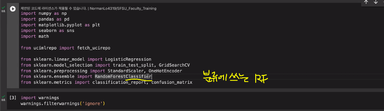

학생 퍼포먼스 분류 모델

# fetch dataset
student_performance = fetch_ucirepo(id=320)

# data (as pandas dataframes)
X = student_performance.data.features
y = student_performance.data.targets
X.head()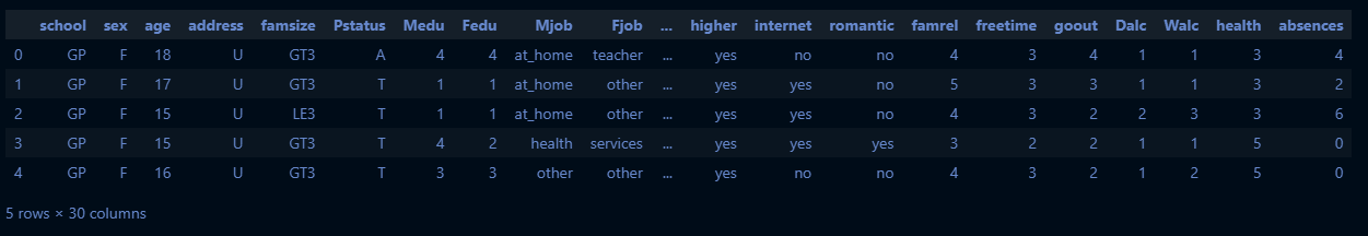

# 변수 정보
student_performance.variables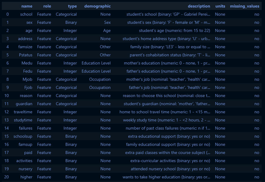

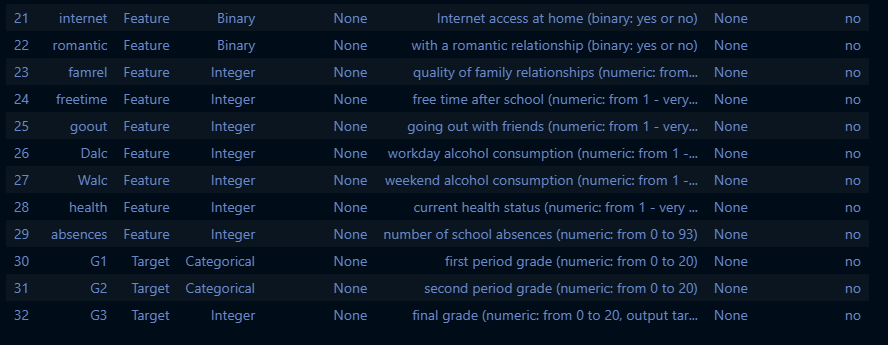
# 분류 문제를 위한 데이터 전처리
## 3번의 시험 등수를 합산해서 A(상위), B(중위), C(하위)등급으로 분류
## A: 상위 ~20%, B: 상위 20~70%, C: 상위 70%~

y['total'] = y.sum(axis=1)
y_a_cut = y['total'].quantile(0.8)
y_b_cut = y['total'].quantile(0.3)

print((y_a_cut, y_b_cut))

[실행 결과]
(42.0, 30.0)

y['grade'] = np.where(y['total'] >= y_a_cut, 'A', np.where(y['total'] >= y_b_cut, 'B', 'C'))
y.head()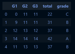

# 로지스틱 회귀를 위해 X 범주형 변수를 더미화
categorical_cols = X.select_dtypes(include=['object', 'category']).columns
X_dummy = pd.get_dummies(X, columns=categorical_cols, drop_first=True)
X_dummy.head()

X_dummy.columns

[실행 결과]
Index(['age', 'Medu', 'Fedu', 'traveltime', 'studytime', 'failures', 'famrel',
       'freetime', 'goout', 'Dalc', 'Walc', 'health', 'absences', 'school_MS',
       'sex_M', 'address_U', 'famsize_LE3', 'Pstatus_T', 'Mjob_health',
       'Mjob_other', 'Mjob_services', 'Mjob_teacher', 'Fjob_health',
       'Fjob_other', 'Fjob_services', 'Fjob_teacher', 'reason_home',
       'reason_other', 'reason_reputation', 'guardian_mother',
       'guardian_other', 'schoolsup_yes', 'famsup_yes', 'paid_yes',
       'activities_yes', 'nursery_yes', 'higher_yes', 'internet_yes',
       'romantic_yes'],
      dtype='object')

# 데이터 전처리 및 분할
y = y['grade']
X_train, X_test, y_train, y_test = train_test_split(X_dummy, y, test_size=0.2, random_state=42)

X_train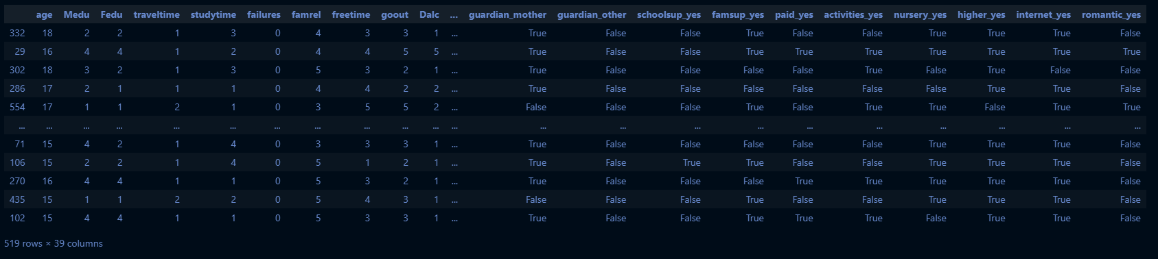

로지스틱 회귀 분류

# 모델 학습
## 다중 클래스 분류를 위해 multi_class 설정
log_reg = LogisticRegression(multi_class="ovr", solver="lbfgs")
log_reg.fit(X_train, y_train)

# 모델 성능 확인
y_pred_log = log_reg.predict(X_test)
print(classification_report(y_test, y_pred_log))

[실행 결과]
              precision    recall  f1-score   support

           A       0.45      0.28      0.34        36
           B       0.60      0.75      0.67        69
           C       0.52      0.44      0.48        25

    accuracy                           0.56       130
   macro avg       0.53      0.49      0.50       130
weighted avg       0.54      0.56      0.54       130

macro: 전체
weighted: 가중치 적용

log_reg2 = LogisticRegression(multi_class="multinomial", solver="lbfgs")
log_reg2.fit(X_train, y_train)
y_pred_log2 = log_reg2.predict(X_test)
print(classification_report(y_test, y_pred_log2))

[실행 결과]
              precision    recall  f1-score   support

           A       0.52      0.33      0.41        36
           B       0.59      0.72      0.65        69
           C       0.50      0.44      0.47        25

    accuracy                           0.56       130
   macro avg       0.54      0.50      0.51       130
weighted avg       0.55      0.56      0.55       130

랜덤 포레스트 모델

# 랜덤 포레스트 모델 생성 및 학습
rf = RandomForestClassifier(n_estimators=100, random_state=1)
rf.fit(X_train, y_train)

y_pred_rf = rf.predict(X_test)
print(classification_report(y_test, y_pred_rf))

[실행 결과]
              precision    recall  f1-score   support

           A       0.56      0.14      0.22        36
           B       0.58      0.84      0.69        69
           C       0.48      0.40      0.43        25

    accuracy                           0.56       130
   macro avg       0.54      0.46      0.45       130
weighted avg       0.55      0.56      0.51       130

# 하이퍼파라미터 튜닝 - Grid Search 정의
param_grid = {
    'n_estimators': [50, 100, 200],  # 트리 개수
    'max_depth': [10, 20, 30],  # 트리 최대 깊이
    'min_samples_split': [2, 5, 10],  # 내부 노드 분할을 위한 최소 샘플 수
    'min_samples_leaf': [2, 5, 10]  # 리프 노드의 최소 샘플 수
}

grid_search = GridSearchCV(
    estimator=RandomForestClassifier(random_state=1),
    param_grid=param_grid,
    cv=5,  # 5-fold 교차 검증
    n_jobs=-1,  # 모든 코어 사용
    verbose=2  # 진행 상황 출력
)

# Grid Search 수행
grid_search.fit(X_train, y_train)

# 최적 파라미터 및 성능 출력
print("Best parameters:", grid_search.best_params_)
print("Best cross-validation score:", grid_search.best_score_)

[실행 결과]
Fitting 5 folds for each of 81 candidates, totalling 405 fits
Best parameters: {'max_depth': 10, 'min_samples_leaf': 2, 'min_samples_split': 2, 'n_estimators': 50}
Best cross-validation score: 0.6320014936519791

rf_best = grid_search.best_estimator_
y_pred_rf_best = rf_best.predict(X_test)
print(classification_report(y_test, y_pred_rf_best))

[실행 결과]
              precision    recall  f1-score   support

           A       0.40      0.06      0.10        36
           B       0.56      0.87      0.68        69
           C       0.56      0.40      0.47        25

    accuracy                           0.55       130
   macro avg       0.51      0.44      0.41       130
weighted avg       0.52      0.55      0.48       130

# Feature Importance
feature_importance = pd.Series(rf_best.feature_importances_, index=X_train.columns).sort_values(ascending=False)
print(feature_importance)

[실행 결과]
failures             0.107221
Fedu                 0.053832
absences             0.053627
Walc                 0.049068
health               0.048440
age                  0.045890
Medu                 0.041877
freetime             0.041875
goout                0.040356
studytime            0.040330
higher_yes           0.035856
school_MS            0.035289
traveltime           0.032885
Dalc                 0.030089
famrel               0.030075
sex_M                0.023730
guardian_mother      0.021508
Mjob_other           0.018171
activities_yes       0.017792
address_U            0.017603
internet_yes         0.017205
reason_reputation    0.017070
romantic_yes         0.016691
famsize_LE3          0.016114
Fjob_services        0.016066
schoolsup_yes        0.016017
famsup_yes           0.015588
Fjob_other           0.013288
nursery_yes          0.012530
reason_home          0.011244
Mjob_services        0.010950
Mjob_teacher         0.010686
Mjob_health          0.009765
reason_other         0.008831
Pstatus_T            0.006961
guardian_other       0.004924
paid_yes             0.003909
Fjob_health          0.003428
Fjob_teacher         0.003219
dtype: float64

# 모델 일반화 성능을 높이기 위해 Feature의 일부만 사용

selected_feature = feature_importance.iloc[:15].index.tolist()
X_train_selected = X_train[selected_feature]
X_test_selected = X_test[selected_feature]

rf2 = RandomForestClassifier(random_state=1, **grid_search.best_params_)
rf2.fit(X_train_selected, y_train)

y_pred_rf2 = rf2.predict(X_test_selected)
print(classification_report(y_test, y_pred_rf2))

[실행 결과]
              precision    recall  f1-score   support

           A       0.75      0.08      0.15        36
           B       0.56      0.88      0.69        69
           C       0.56      0.40      0.47        25

    accuracy                           0.57       130
   macro avg       0.62      0.46      0.43       130
weighted avg       0.61      0.57      0.50       130

grid_search2 = GridSearchCV(
    estimator=RandomForestClassifier(random_state=1),
    param_grid=param_grid,
    cv=5,  # 5-fold 교차 검증
    n_jobs=-1,  # 모든 코어 사용
    verbose=2  # 진행 상황 출력
)

# Grid Search 수행
grid_search2.fit(X_train_selected, y_train)

# 최적 파라미터 및 성능 출력
print("Best parameters:", grid_search2.best_params_)
print("Best cross-validation score:", grid_search2.best_score_)

[실행 결과]
Fitting 5 folds for each of 81 candidates, totalling 405 fits
Best parameters: {'max_depth': 20, 'min_samples_leaf': 5, 'min_samples_split': 2, 'n_estimators': 200}
Best cross-validation score: 0.6320014936519791

rf_best2 = grid_search2.best_estimator_
y_pred_rf_best2 = rf_best2.predict(X_test_selected)
print(classification_report(y_test, y_pred_rf_best2))

[실행 결과]
              precision    recall  f1-score   support

           A       1.00      0.06      0.11        36
           B       0.56      0.88      0.69        69
           C       0.58      0.44      0.50        25

    accuracy                           0.57       130
   macro avg       0.71      0.46      0.43       130
weighted avg       0.69      0.57      0.49       130

Suhyeon Lee

2 B R 0 2 B

이전 포스트

머신 러닝 빌드업 - 3회차

다음 포스트

머신러닝 특강: 분류 분석

라이브 세션

목표

분류 모델

정의

성능 지표

분류 모형

로지스틱 회귀 분석 (Logistic Regression)

정의

모델 설명

다중 클래스 분류

랜덤 포레스트

정의

의사결정나무(Decision Tree)

앙상블(Ensemble)

랜덤 포레스트(Random Forest)

실습

학생 퍼포먼스 분류 모델

로지스틱 회귀 분류

랜덤 포레스트 모델

머신 러닝 빌드업 - 3회차

머신 러닝 특강: 회귀 분석

0개의 댓글

관련 채용 정보