FPCV 2주차, Image Sensing, Binary Images

개요

• First Principles of Computer Vision 스터디 정리용 글
• 2주차는 image sensing과 binary images까지 들음

Image Sensing

Overview

• Video Link
• topics
  - history of imaging
  - types of image sensors
  • resolution, noise, dynamic range
  • sensing color
  • camera response and HDR imaging
  • nature's image sensors

Brief History of Imaging

• Video Link
• Pinhole Camera (1558), Camera Obscura
• Lens Based Camera Obscura (1568), sketch by human
• Invention of Film (1837), still hard to get high-resolution, colorful image
• Color Film (1877)
• Ernemann Camera (1928), 'What You Can See You Can Photograph', Personal Camera
• Silicon Image Detector (1970) --> Digital Cameras (1975) --> Phones with Cameras, iPhone 1 (2000)
• The era of Visual Communication (SnapChat, Instagram, Youtube, Tiktok)

Types of Image Sensor

• Video Link
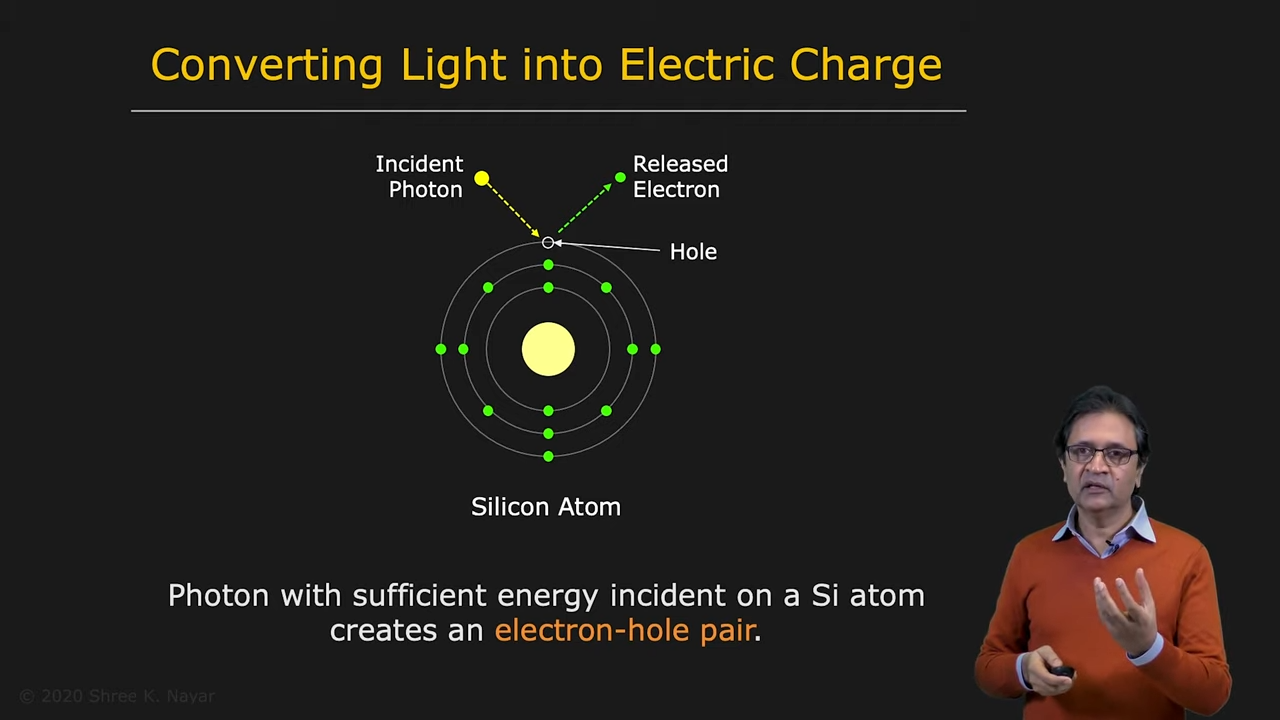
• Converting Light into Electric Charge

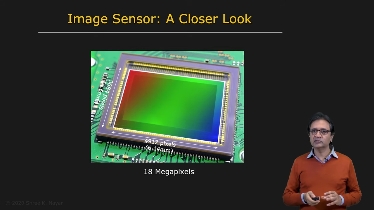
실리콘의 전자구조	이미지 센서의 예시

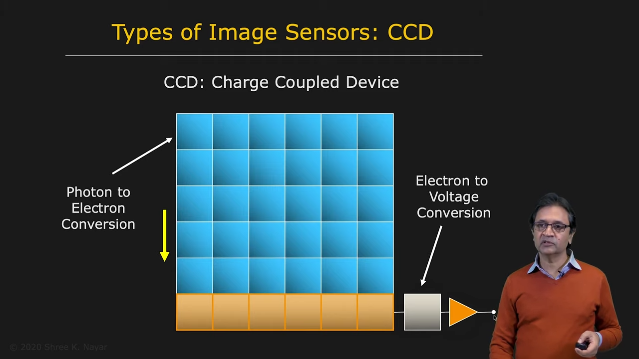
• Charge Coupled Device (CCD) : Bucket Brigade처럼 Photon -> Electron -> Voltage로 Conversion
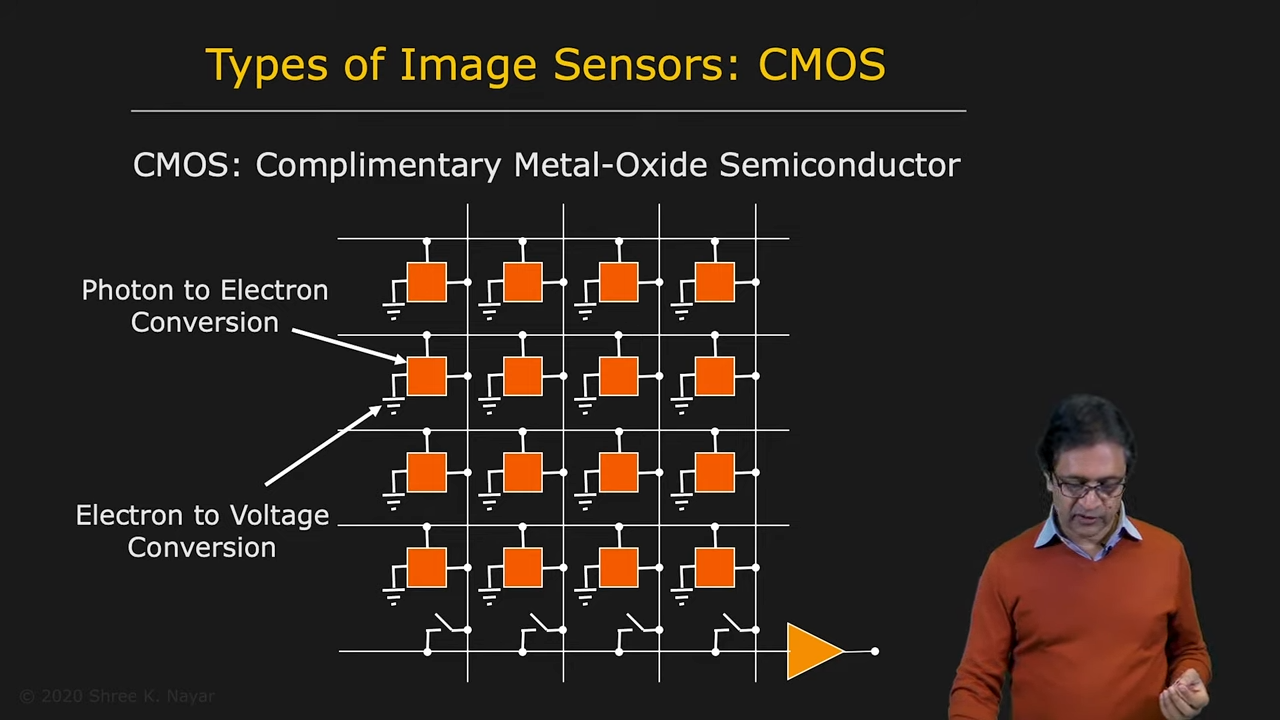
• Complimentary Metal-Oxide Semiconductor (CMOS) : 각각의 pixel의 값만 읽어올 수 있어서 훨씬 유연한 사용이 가능

CCD의 구조	CMOS의 구조

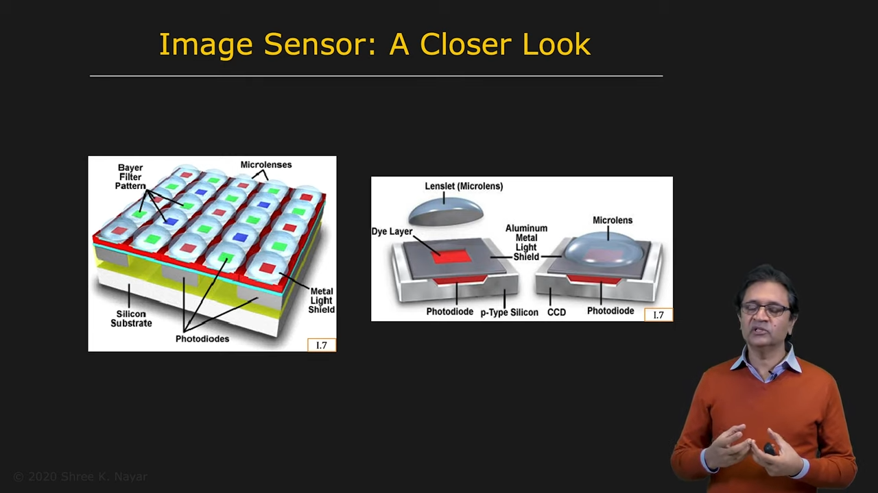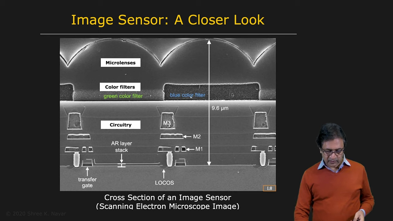Color Filter와 Lens를 활용한 Image Sensor	Image Sensor의 수직 단면

Resolution, Noise, Dynamic Range

• Video Link
• Resolution을 높이기 위해 센서를 배치시키는 것도 어렵지만 전력도 더 많이 먹어서 해결해야할 문제가 많았다
• Noise는 Capture, Conversion, Transmission, Processing의 과정에서 signal에 끼는 unwanted modification
• Noise의 원인들
  • Photon Shot Noise (Scene Dependent) : Quantum nature of light, Random arrival of photons
  • Readout Noise (Scene Independent) : Electronic Noise (Pre analog-to-digital conversion), Quantization Noise (Post analog-to-digital)
  • Other Sources (Scene Independent): Dark Current Noise (e.g. the light from thermal), Fixed Pattern Noise (Manufactured Pixel Noise)
• Noise를 Modeling하는 방법들
  • Photon Noise : Poisson Distribution (아무런 정보가 없는 경우 유용하게 사용될 수 있는 Distribution)
  • Read Noise : Gaussian Distribution (high-quality sensor -> low std, low-quality sensor -> high std)
  • Quantization Noise : 충분히 큰 bit (12-14) 정도면 무시할 수 있다
  • Dark Current Noise (Thermal) : Poisson Distribution을 따르며 Long Exposures일 때만 영향을 끼친다 (e.g. 2 mins on astronomy) 비싼 cooling system을 이용해 영향을 최소화 한다
  • Fixed Pattern Noise (Defective Pixels) : calibration 단계에서 이를 보정할 수 있다
• Sensor Dynamic Range : Noise에 강인한 정도와 흡수할 수 있는 광자의 에너지에 따라서 정해진다

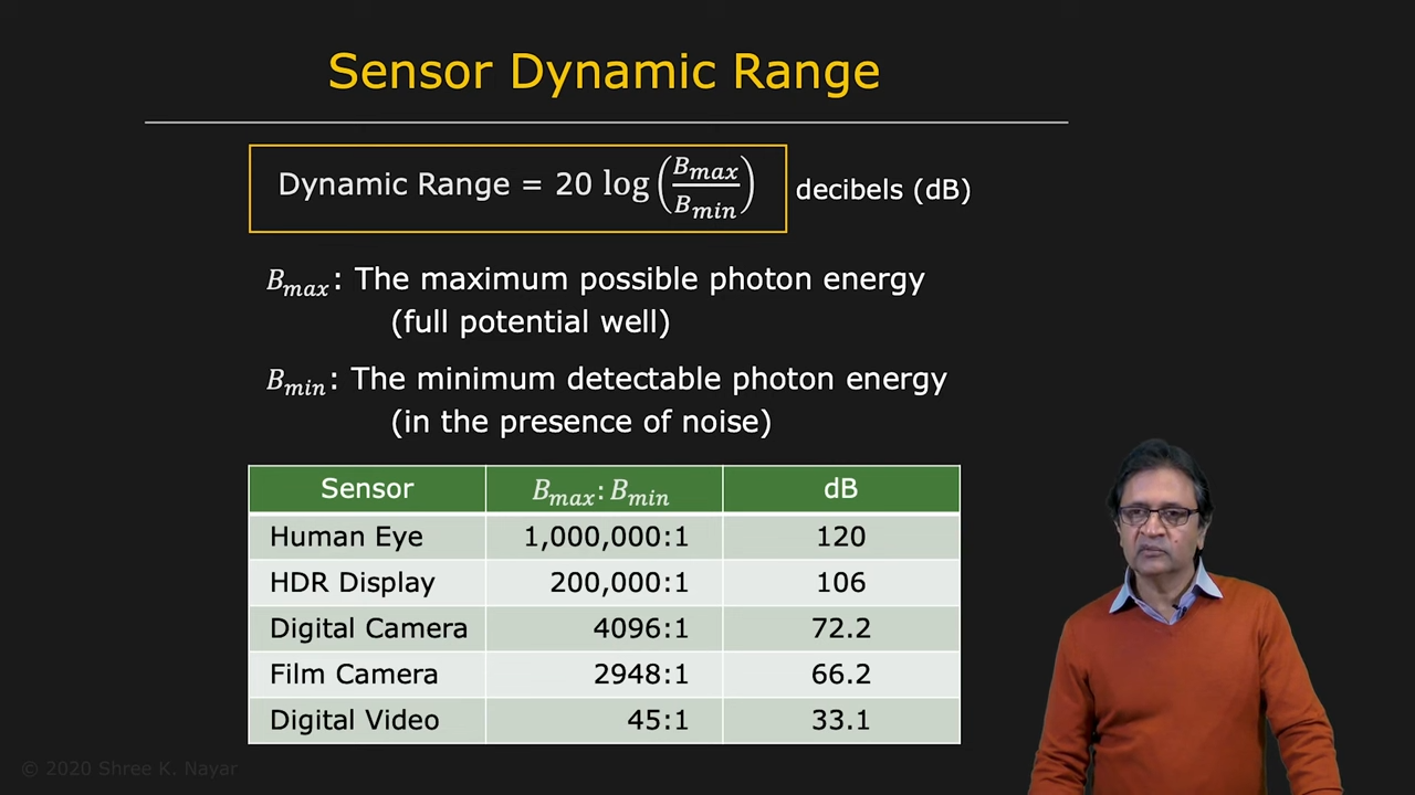다양한 센서의 Dynamic Range

Sensing Color

• Video Link
• Quantum Efficiency : Wavelength에 따라 빛은 다양하게 들어올 수 있다. 이를 얼마나 정확하게 반영해서 electron flux로 변환할 수 있는가에 대한 지표라고 할 수 있다

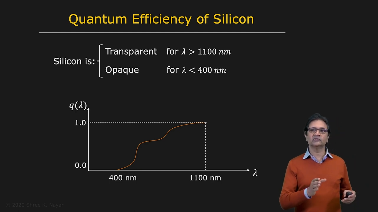Silicon은 거의 완벽한 quantum efficiency를 가지고 있다

• Monochromatic Light라고 하더라도 Spectral Distribution을 가지고 있을 수 있다. 이를 확률분포 적분을 통해 기댓값을 얻을 수 있다. 이때 probability function은 color filter를 활용해서 구현할 수 있다
• 이 때 적분이 continuous하기 때문에 infinite color filter를 필요로 할 것 같지만, 나중에 자세히 보겠지만 생각보다 적은 수의 color filter로도 정보를 잃지 않을 수 있다
• Color란 무엇인가? 서로다른 wavelength들에 대한 "human response"이다. 400nm (Violet) to 700nm (Red) 정도의 가시광선 영역.
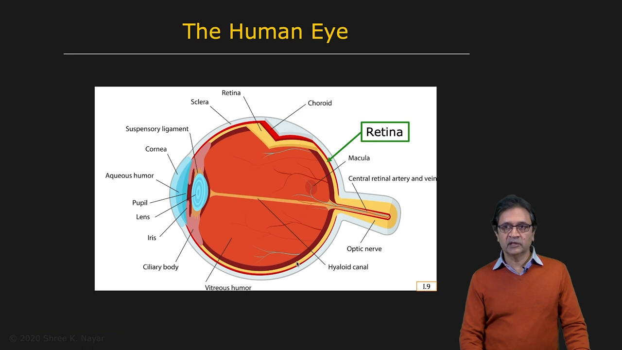
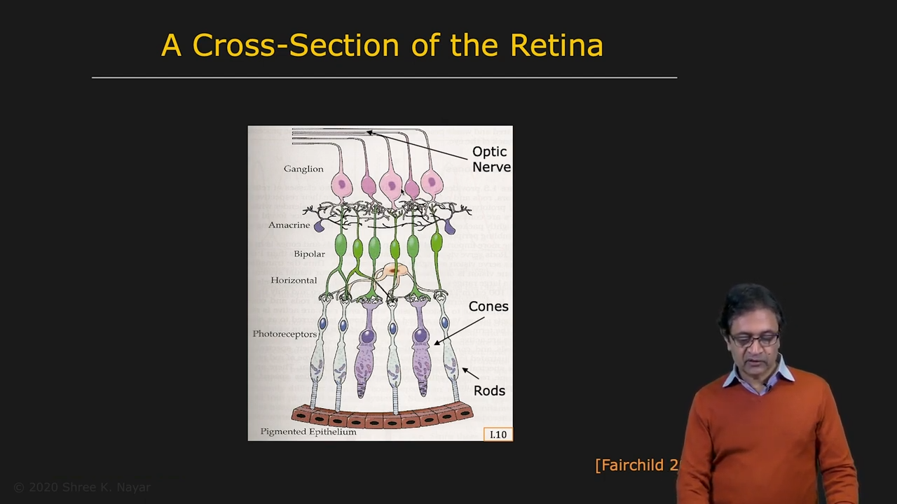
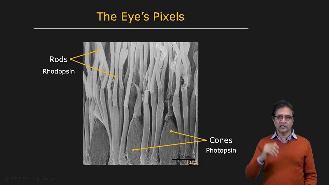
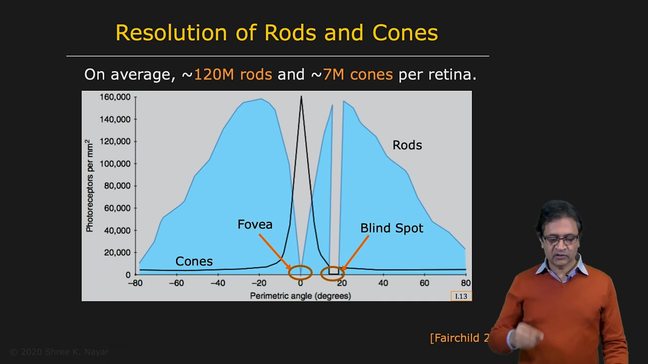
• 우리도 spectral distribution을 전부 복구하는가? 사람의 시각 센서들인 Rods & Cones를 살펴보면 그렇지 않다. Rod는 rhodopsin을 가지고 있어서 적은 양의 빛에도 반응할 수 있고(schotopic vision), Cone은 Photopsin을 가지고 있어서 빛이 강할 때 색을 구별할 수 있다(photopic vision).

눈 구조	retina의 구조	Rods & Cones

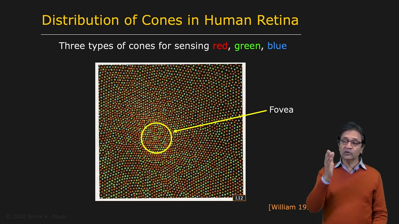
retina의 pixel 구조	rod들과 cone들의 분포

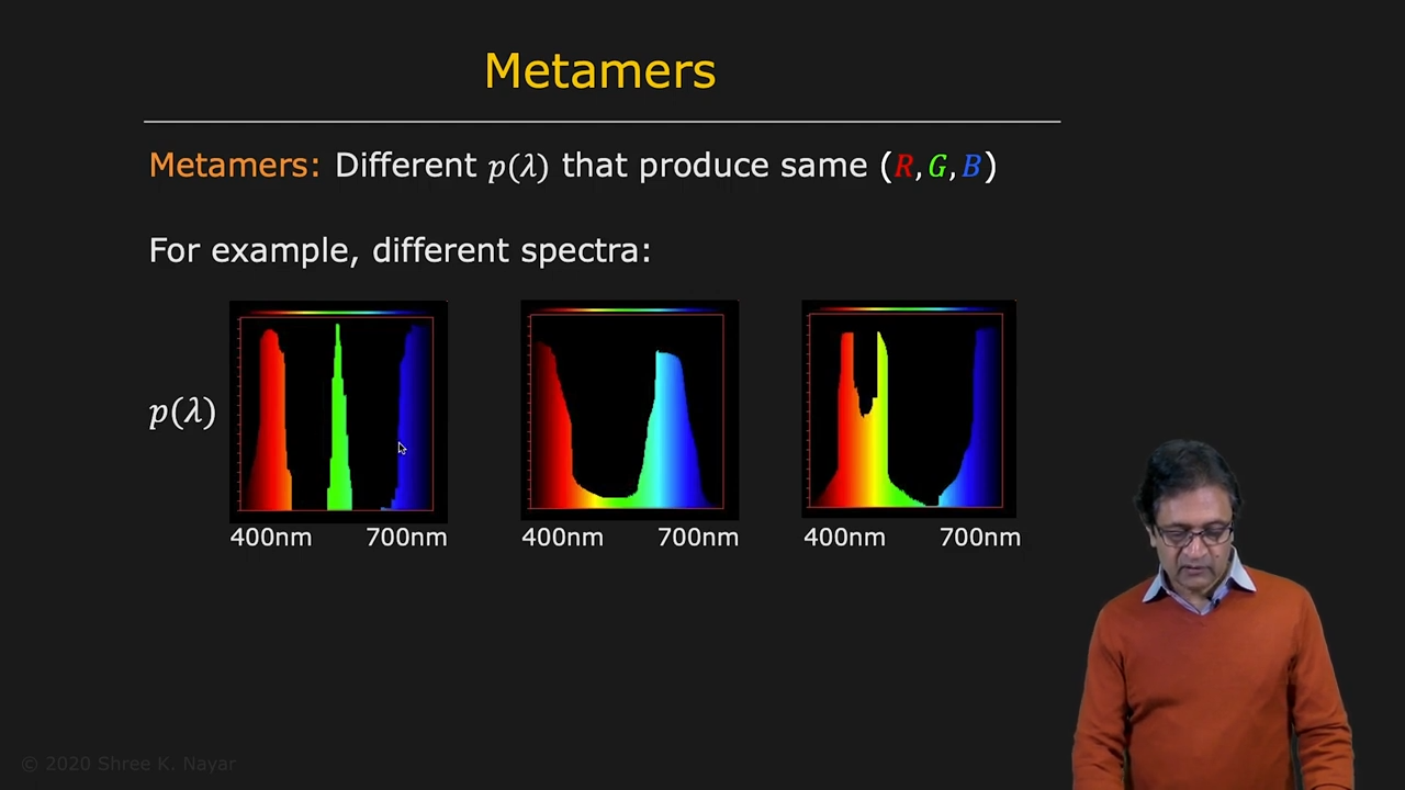
서로 다른 p들로도 동일한 RGB 시스템을 구성할 수 있다, 색을 섞어서 인식할 수 있기 때문

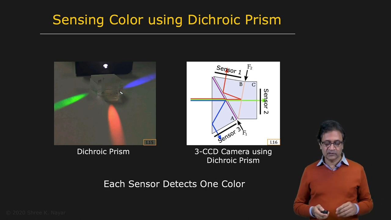
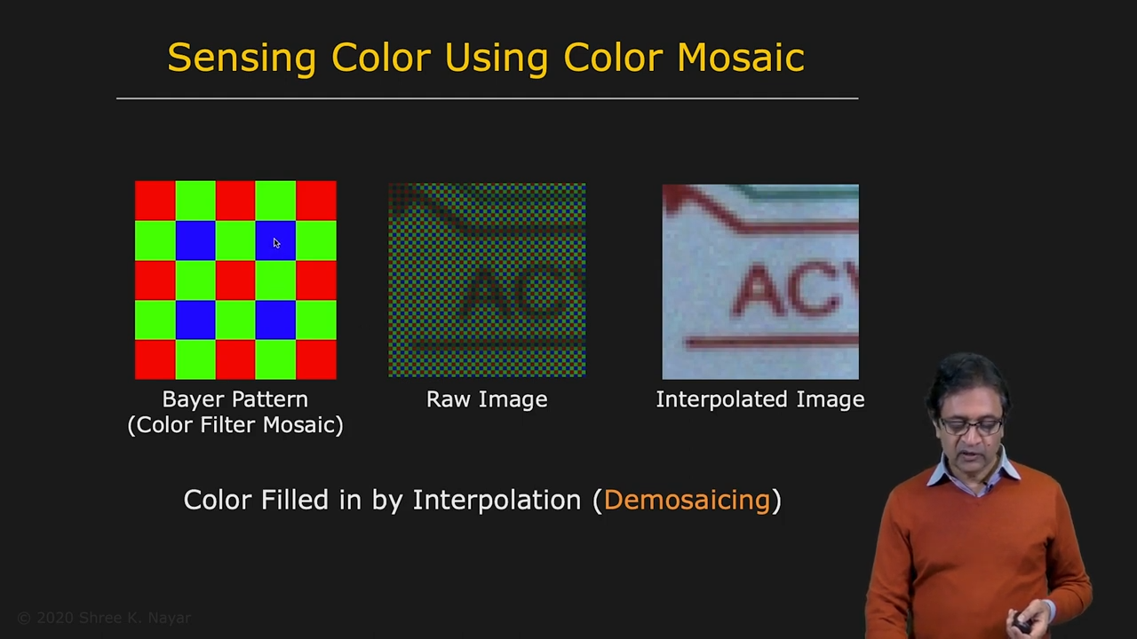
Sensing Color using Dichroic Prism	Sensing Color using Color Mosaic (Bayer Pattern)

Camera Response and HDR Imaging

• Videi Link
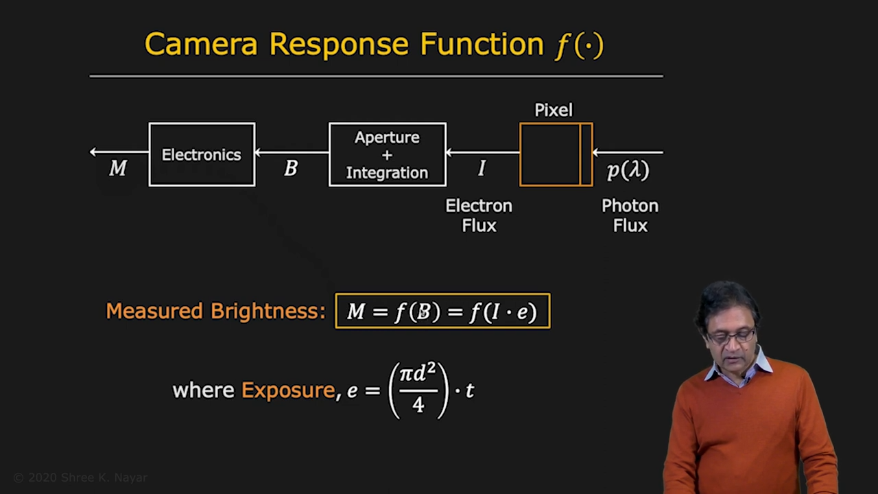
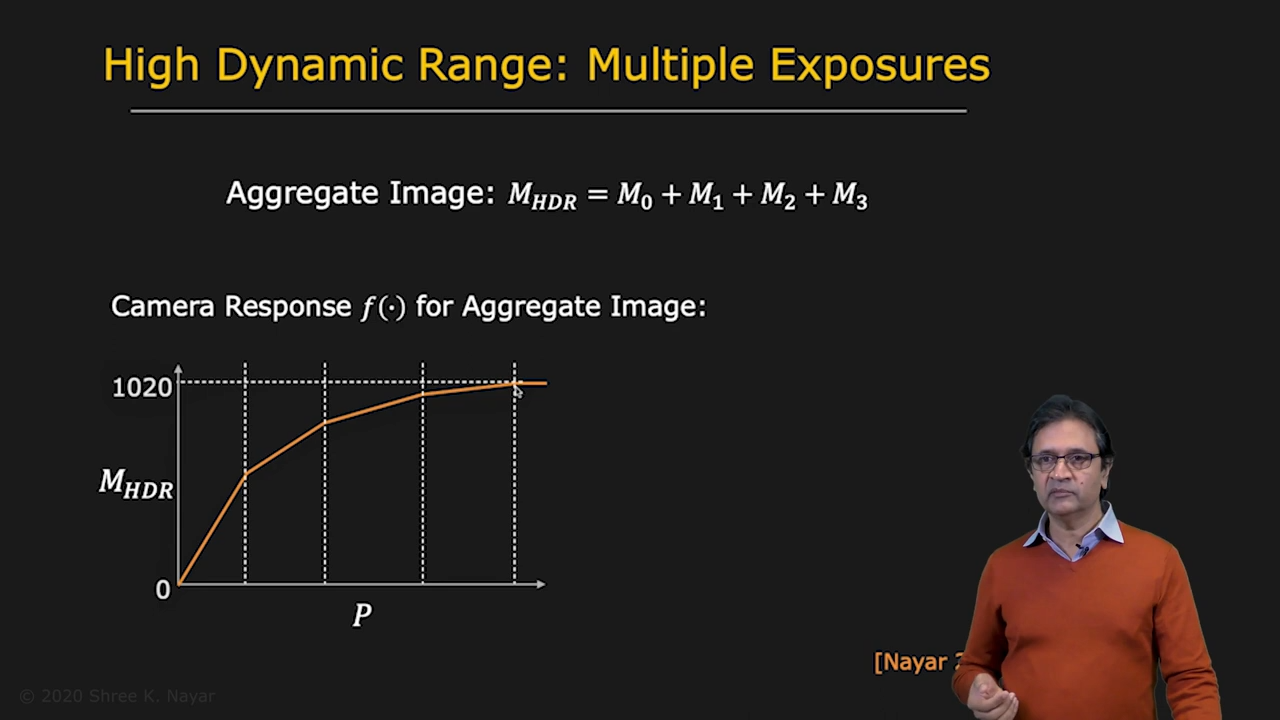
• Scene Brightness와 Image Brightness는 linear하지 않다. 우리가 원하는 이미지를 얻기 위해서는 Camera Response Function F를 통해서 Electron Flux들을 Aperture와 Temporal Integration를 통해 원하는 brightness를 얻어낸다
• 마지막으로 다양한 Process를 거쳐서 우리가 원하는 Image를 얻어낸다

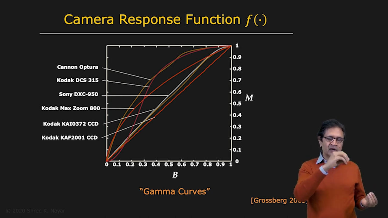
Theoritical Camera Response Function	Camera Response Function f in Real Cameras

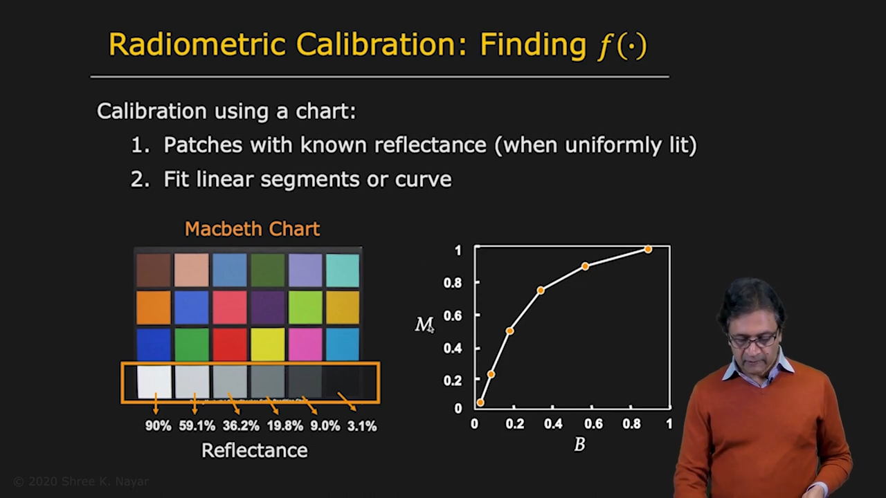
Macbeth Chart의 Reflectance Row를 통해서 이를 역산할 수 있다

• 이를 역산하는 것을 radiometric calibration이라 부른다
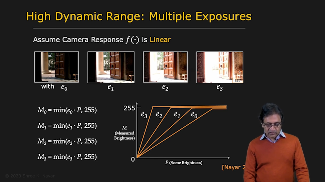
• High Dynamic Range (HDR)
  • 현실에는 outlier brightness를 가진 scene과 object가 많이 존재한다 (e.g. sky, sun)
  • Exposure의 조절을 통해서 이를 제어할 수 있다

이런 여러 exposure의 결과물을 동시에 활용할 수 있다면?	naive interpolation의 결과물

• 문제는 이런 경우 Motion이 있는 scene을 잡아내기 어렵다 (여러 번 exposure 했기 때문에)
• single shot HDR Imaging은 어떻게 구현할 수 있을까? -> Sensor 위에 different exposure를 위한 filter를 씌운다

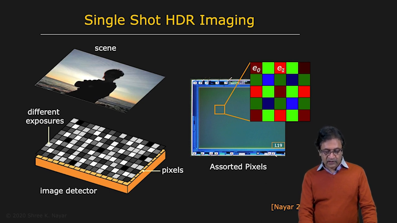Single Shot HDR idea

Nature's Image Sensors

• Video Link
• Copilia의 눈은 두개의 lens와 한 개의 sensor를 가지고 있다.
• Brittle Star(거미 불가사리)는 몸 전체가 lense들로 뒤덮여 있다
• Octopus(문어)의 Camouflage, 이들은 질감과 색감을 바꿀 수 있다
• Human Eye에는 Blind Spot도 있고 Rods&Cones도 빛에서 반대 방향으로 꺽여있다. 이 모든 문제들을 뇌가 processing 해준다

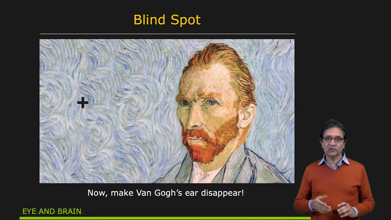왼쪽 눈을 가리고 십자가에 주목하면서 반고흐를 지우기가 가능한가? 너무 큰데...

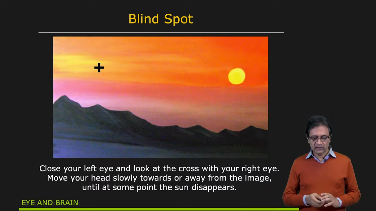해를 없애는 건 상대적으로 쉽다

• 근데 사실상 눈 두개면 동시에 blind spot에 들어가긴 거의 불가능한 거 같기도?

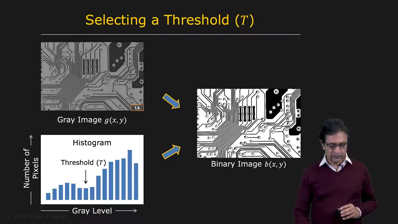
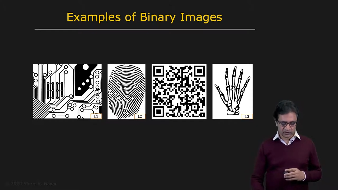
Binary Images

Overview

• Video Link

요즘은 잘 안 쓰지만 robust한 computer vision system을 만드는데 매우 유용하다	예시	예시2 (QR Code 포함)

• 3D에서도 stable configuration를 prior로 활용한다면 object classification 등에 활용될 수 있다
• Geometric Properties
• Segmenting Binary Images
• Iterative Modification : Skeleton을 뽑는데 사용할 수 있다

Geometric Properties

• Video Link
• binary image는 continuous하고 하나의 object만 있다는 가정을 가진다면 면적분을 통해 Area (Zero Moment)를 쉽게 구해낼 수 있다. 기댓값 면적분을 통해 Position (First Moment)도 쉽게 구해낼 수 있다.
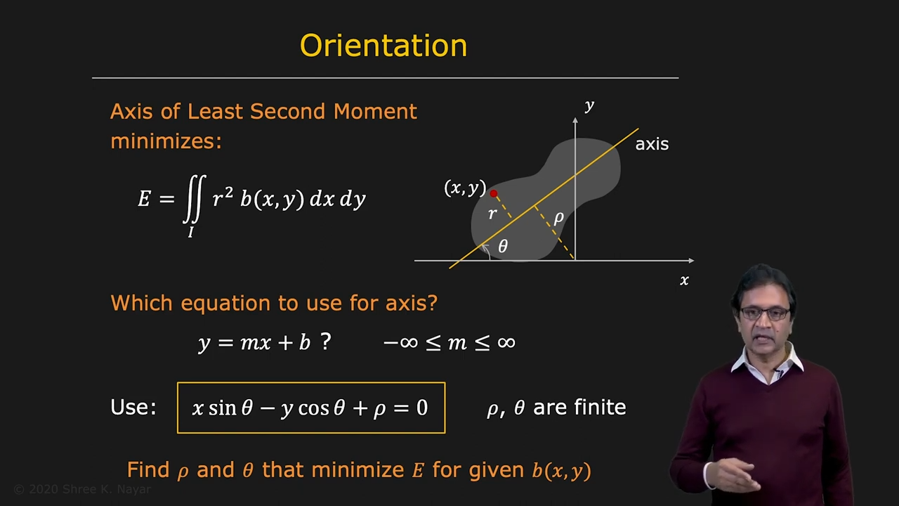
• Orientation은 어떻게 정의할 수 있을까? Axis of Least Second Moment

second moment를 최소화 하는 직선의 기울기를 찾으면 된다

• minimization의 방향성
• (1) 미분값이 0이 되는 지점을 찾는게 목표
• (2) 원점으로 coordinate system을 옮기자
• (3) 서로 직각하는 두개의 theta의 해를 찾을 수 있으며 각각 minimum E와 maximum E를 준다
• (4) 직접 넣어보거나 second derivative test를 진행할 수 있다
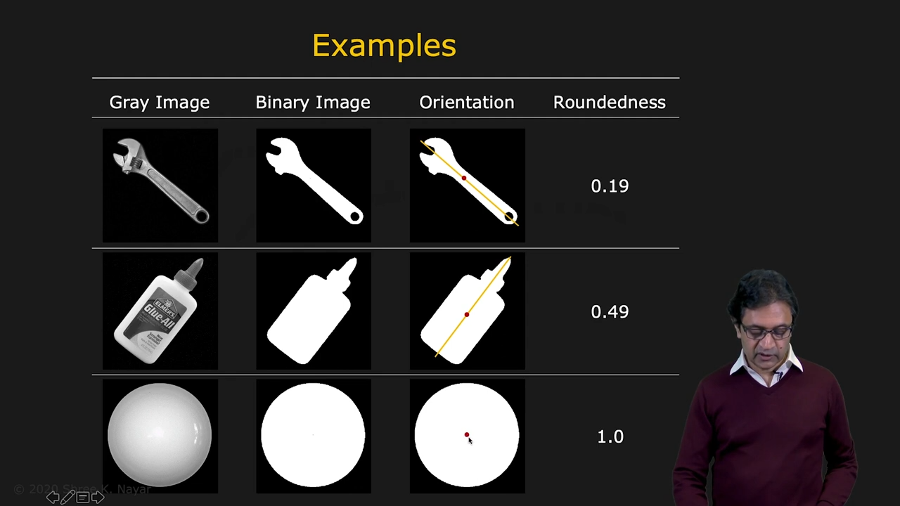
• Roundedness는 어떻게 정의할 수 있을까? max E와 min E의 이심률로 정의할 수 있다

예시, 이런 feature들을 이용해 classification도 할 수 있다

• Discrete Binary Images에서도 Area, Position, Orientation, Roundedness를 동일한 방식으로 구할 수 있다. 연속 적분을 이산 합으로 바꾸기만 하면!

Segmenting Binary Images

• Video Link
• 이제 multiple object들이 있다고 생각하면 우리는 component를 구별할 수 있어야함
• connected component : A와 B를 연결하는 b(x,y)가 상수인 path가 존재한다면 connected component
• Region Growing Algorithm
  • (a) Fine unlabeled "seed" point with b = 1. If not found, terminate
  • (b) Assign new label to seed point
  • (c) assign same label to its neighbors with b = 1
  • (d) assign same label to neighbors of neighbors with b = 1. repeat until no more unlabeld neighbors with b = 1.
  • (e) go to (a)
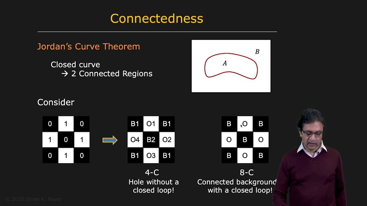
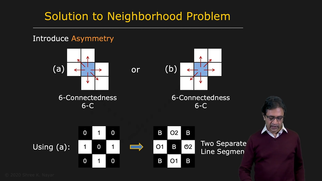
• connectedness : 4 neighbors vs 8 neighbors, 둘다 완벽하지 않다
• Jordans' Curve Theorem : Closed curve는 2 Connected Regions을 만든다

이런 minimal example만 봐도 둘다 완벽하지 않음	Hexagonal Tessellation과 비슷한 효과를 주는 해결책, 4 neighbors

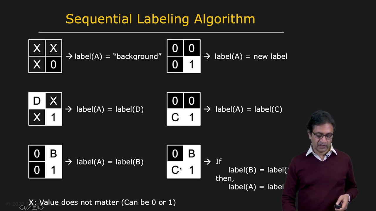
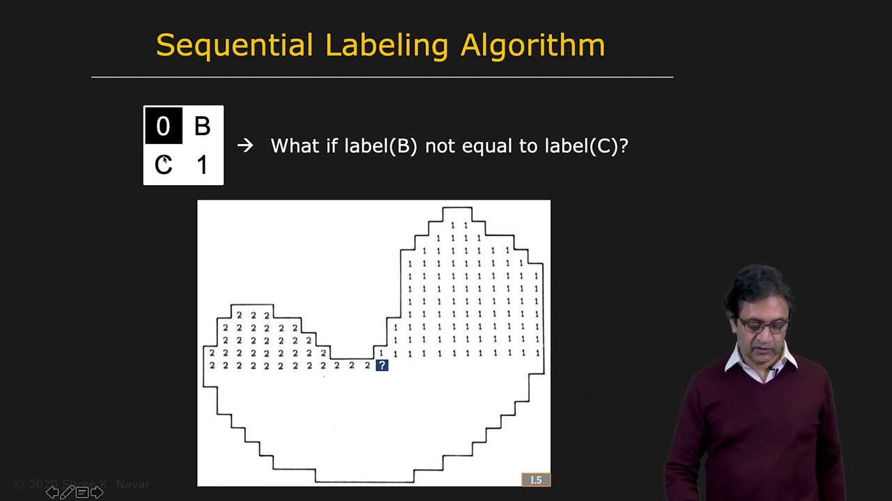
• sequential labeling algorithm : with window we can rasterize the labeling

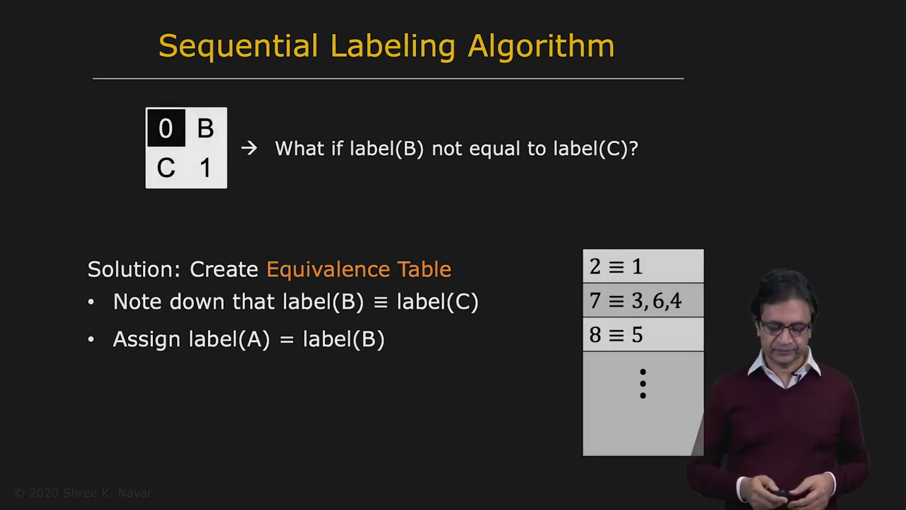2x2 window의 경우	한계	Equivariance Table을 이용한 해결

Iterative Modification

• Video Link
• example : human body to skelecton

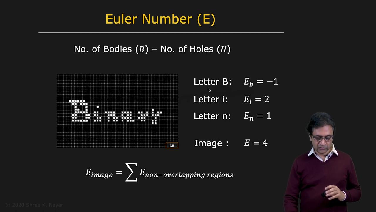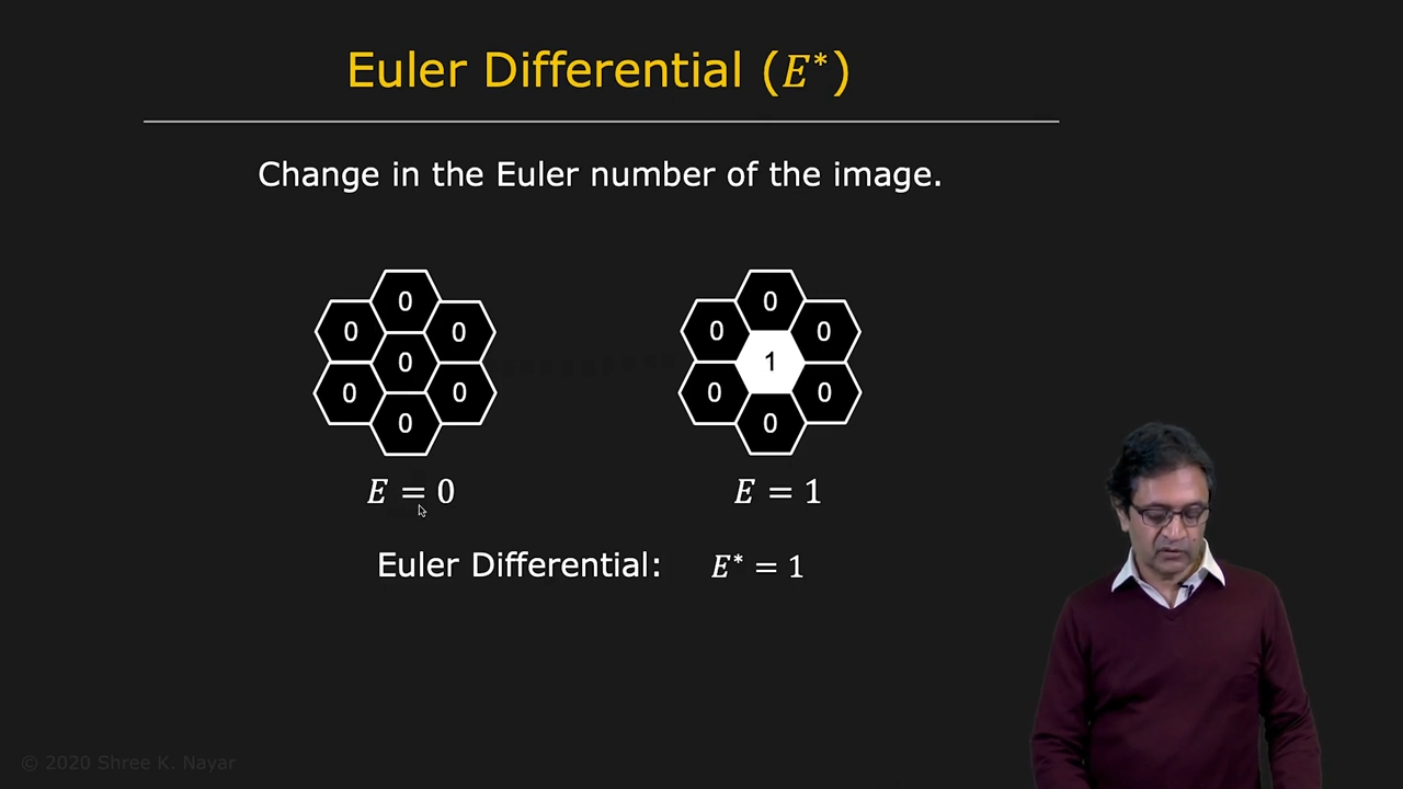위상 수학의 eluer number E	eluer differential

• neighborhood를 eluer differential을 활용해서 정하면 independent rasterization이 가능하다
• iterative하게 몇 번 적용함으로써 optimal한 skeleton에 도달할 수 있다

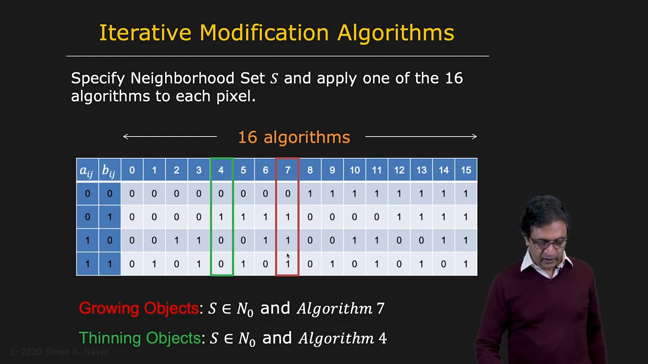값의 mapping에 따라서 object를 키우거나 줄이는 일이 가능하다