혼공 ML+DL #22

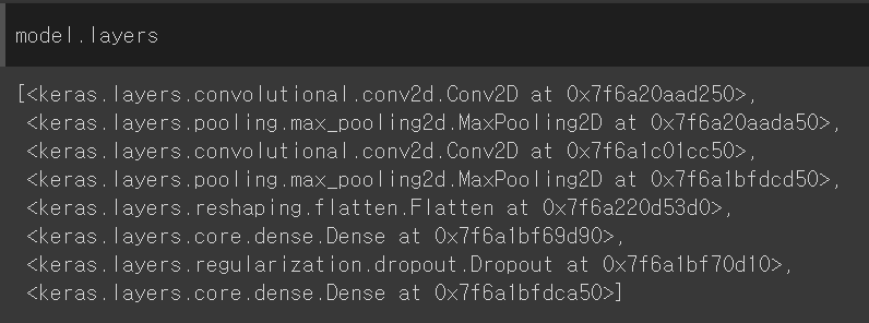
• 모델 layers
  8개의 객체를 리스트로 가짐

• conv 층의 가중치 크기 확인
  weights[0] = 가중치, weights[1] = 절편

conv = model.layers[0]
print(conv.weights[0].shape, conv.weights[1].shape)

(3, 3, 1, 32) (32,)
-> 3x3x1 필터 32개

📌 층의 가중치 시각화

📍 1. 히스토그램

• 가중치 값의 분포 (3x3x1x32 개)

conv_weights = conv.weights[0].numpy()

import matplotlib.pyplot as plt
plt.hist(conv_weights.reshape(-1, 1))
plt.xlabel('weight')
plt.ylabel('count')
plt.show()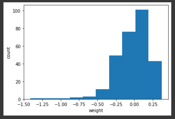

📍 2. 3x3 이미지

• vmin보다 작은 값은 vmin으로, vmax보다 큰 값은 vmax로

fig, axs = plt.subplots(2, 16, figsize=(15,2))

for i in range(2):
    for j in range(16):
        axs[i, j].imshow(conv_weights[:,:,0,i*16 + j], vmin=-0.5, vmax=0.5)
        axs[i, j].axis('off')

plt.show()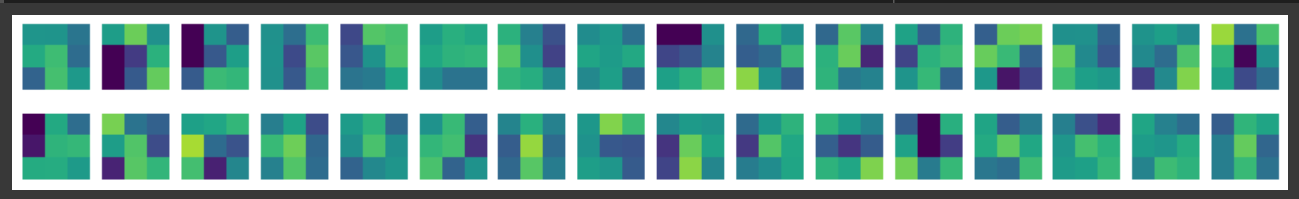

📌 Functional API

• 합성곱 층의 활성화 출력 시각화

• add를 사용하지 않고 함수처럼 호출하여 모델의 층을 자유롭게 조합 가능

• Input() : InputLayer 객체 생성하여 첫 번째 층(dense1)에 입력 필요

• DATA SET

(train_input, train_target), (test_input, test_target) = keras.datasets.fashion_mnist.load_data()
plt.imshow(train_input[0], cmap='gray_r')
plt.show()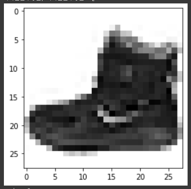

📍 첫 번째 특성 맵 시각화

• conv_acti : Sequential Model 의 input과 첫번째 층 Conv2D 객체의 출력값으로 만든 Model

conv_acti = keras.Model(model.input, model.layers[0].output)

inputs = train_input[0:1].reshape(-1, 28, 28, 1)/255.0
feature_maps = conv_acti.predict(inputs)
print(feature_maps.shape)

(1, 28, 28, 32)

fig, axs = plt.subplots(4, 8, figsize=(15,8))
for i in range(4):
    for j in range(8):
        axs[i, j].imshow(feature_maps[0,:,:,i*8 + j])
        axs[i, j].axis('off')

plt.show()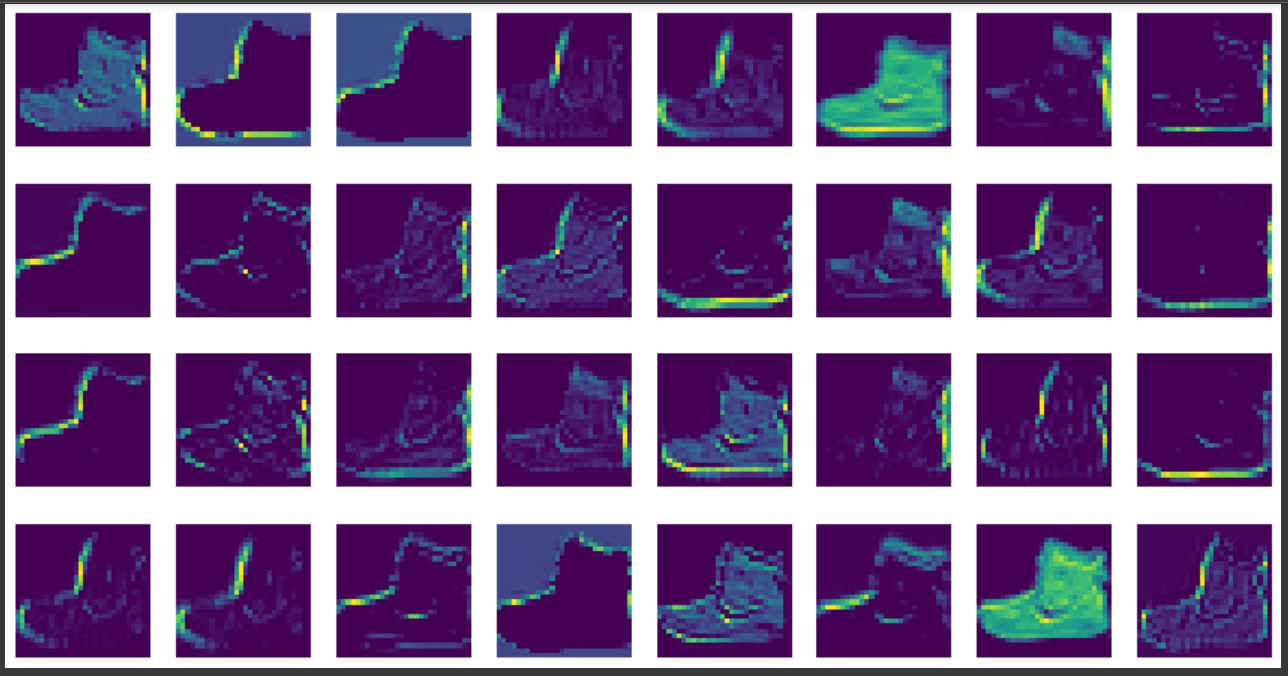

📍 두 번째 특성 맵 시각화

• 두 번째 합성곱 층 : Conv2D -> Maxpooling -> Conv2D_1 이므로 layers[2]
• Maxpooling 으로 크기 1/2 감소
• 64개 (= 필터)

conv2_acti = keras.Model(model.input, model.layers[2].output)
feature_maps = conv2_acti.predict(inputs)
print(feature_maps.shape)

(1, 14, 14, 64)

fig, axs = plt.subplots(8, 8, figsize=(12,12))

for i in range(8):
    for j in range(8):
        axs[i, j].imshow(feature_maps[0,:,:,i*8 + j])
        axs[i, j].axis('off')

plt.show()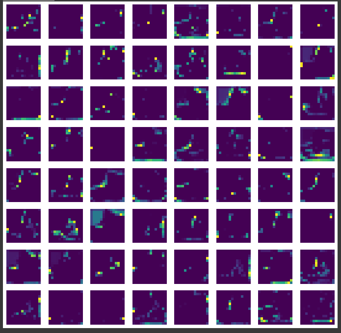

-> 층이 깊어질 수록 고수준 추상적 학습

🔗혼공 MLDL-22