[2주차] 8.10 화

William JO·2021년 8월 15일

Naver Boostcamp AI Tech 2기

목록 보기

7/32

✏️Optimization

Optimization이란?

loss function(L) value가 줄어 들었을 때, 어떤 optimum point에 이룰 것이라 기대; 찾고자 하는 parameter에 대해 L을 편미분한 값을 이용해 학습
Gradient Descent : First-order(1차미분) iterative optimization algorithm for finding a local minimum of a differentiable function

Generalization(일반화)

How well the learned model will behave on unseen data
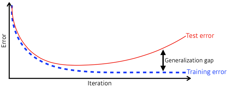
일반적으로 학습 시 training error는 iteration마다 줄어든다.
-> 우리가 원하는 최적값 도달 보장 X
-> 어느 시점부터 test error ↑
generalization gap = generalization performance = 일반화 성능
-> 일반화 성능 좋다해서 모델 성능이 좋다고 보장 X
-> ex) train/test error가 둘다 크지만 gap 없을 경우

Underfitting vs. Overfitting

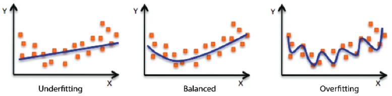
Underfitting : simple network, lack of training, train data도 잘 못 맞춤
Overfitting : train data prediction good, test data prediction bad

Cross-validation(K-fold validation)

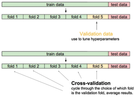
is a model validation technique for assessing how the model will generalize to an independent (test) data set
test data → 학습엔 절대 사용 X (cheating!!)
validation data : over/underfitting 방지 테스트 용
-> 최적의 hyperparameters set을 찾은 후, 고정하고 마지막 학습엔 모든 data를 사용

Bias and Variance

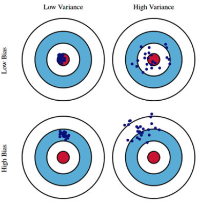
Bias and Variance Tradeoff

Minimizing cost can be decomposed into three different parts: $bias^2$ , variance, and noise
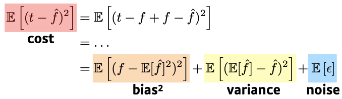
cost를 minimize할 때 근본적으로 train datadp noise가 있다면, bias & variance를 둘 다 줄이기엔 어렵다

Bootstrapping (Ensemble)

is any test or metric that uses random sampling with replacement
학습데이터를 subsampling해서 여러 개 집합을 만들고 그걸로 여러 모델 혹은 metric을 만들어 사용

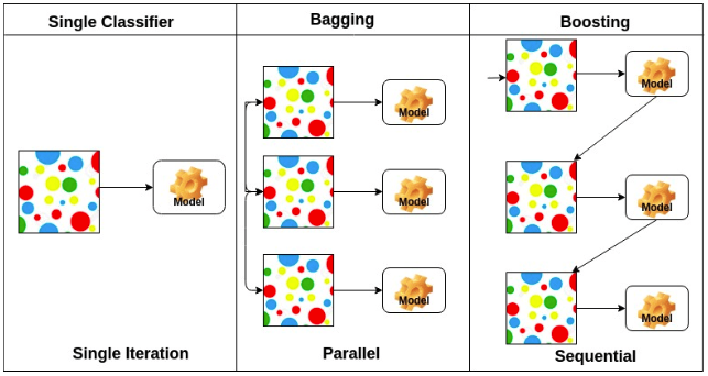
Bagging(Bootstrapping aggregating)
- Multiple models are being trained with bootstrapping.
- ex) Base classifiers are fitted on random subset where individual predictions are aggregated
  (votting or averaging)
- Vanilla 학습보다 성능 ↑
Boosting
- focus on those **specific training samples that are hard to classify
- combine weak learners in sequence where each learner learns from the mistakes of the previous weak learner.
Reference
- https://brunch.co.kr/@chris-song/98
- https://devkor.tistory.com/entry/Ensemble-Methods

✏️Practical Gradient Descent Methods

Gradient Descent Methods

Stochastic GD : Update with the gradinet computed from a single sample(batch-size)
Mini-batch GD : Update with the gradinet computed from a subset of data(batch-size)
Batch GD : Update with the gradinet computed from whole data(batch-size)

Batch-size Matters

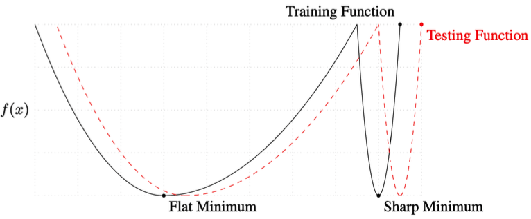
a large batch tend to converge to sharp minimizers while small-batch methods consistently converge to flat minimizers; this is due to the inherent noise in the gradient estimation.
flat minimizer의 generalization performance가 더 좋다.
-> This is why you should use MBGD(flat minimizer)

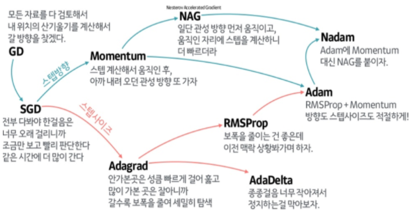
Gradient Descent

$W_{t+1} = W_t - \eta g_t$

$\eta$ : learning-rate, $g_t$ : gradient

문제점 : step-size(lr) 적절히 설정하기 어렵다

Momentum

$a_{t+1} = \beta a_t + g_t$ → momentum이 포함된 gradient로 업데이트
$W_{t+1} = W_t - \eta a_{t+1}$

$\beta$ : momentum, $a_{t+1}$ : accumulation

intuition: 한번 gradient가 ➡방향으로 흐르면, 다음번 grad가 ⬅방향으로 다르게 흘러도, ➡방향 정보를 이어가자. → 전 grad 정보를 활용해보자.

Nesterov Accelerated Gradient(NAG)

$a_{t+1} = \beta a_t + \nabla L(W_t - \eta \beta a_t)$ → $a_t$ 로 이동한 곳에서 gradient를 구한 값으로 $a_{t+1}$ 을 구한다
$W_{t+1} = W_t - \eta a_{t+1}$

$\nabla L(W_t - \eta \beta a_t)$ : Lookahead gradient

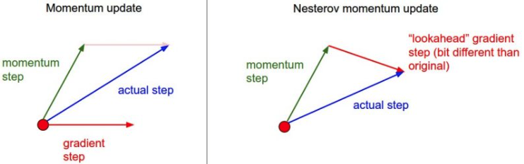
NAG converge가 더 빠르다.

Adagrad

adapts the learning rate, performing larger updates for infrequent and smaller updates for frequent parameters

$W_{t+1} = W_t - \frac{\eta}{\sqrt{G_t + \epsilon}}G_t$

$\epsilon$ : for numerical stability (division by 0 처리)

$G_t$ : sum of gradient squares (t까지의 gradient 변화 저장)

변화 적은 parameter 변화 ⬆, 변화 많은 parameter 변화 ⬇
문제점 : monotonically decreasing = $G_t$ 가 계속 커져서 무한대로 가면 update가 되지 않는다; 뒤로 가면 갈수록 학습 멈춤 현상이 생김

Adadelta

extends Adagrad to reduce its monotonically decreasing the learning rate by restricting the accumulation window → Adagrad의 large $G_t$ 현상을 최대한 막겠다.

$G_t = \gamma G_{t-1} + (1 - \gamma)g_t^2$
$W_{t+1} = W_t - \frac{\sqrt{H_{t-1} + \epsilon}}{\sqrt{G_t + \epsilon}}g_t$
$H_t = \gamma H_{t-1} + (1-\gamma)(\triangle W_t)^2$

$G_t$ : Exponential Moving Average(EMA) of gradient squares

$H_t$ : Exponential Moving Average(EMA) of difference squares

$\frac{\sqrt{H_{t-1} + \epsilon}}{\sqrt{G_t + \epsilon}}$ : Adagrad의 분자로 인한 monotonical decrease를 막는 수식

time의 window-size만큼의 gradient 제곱의 변화를 보겠다.
-> 문제점 : # parameters가 많으면 window-size 무용지물
no learning rate
tuning 힘들어 잘 안쓴다.

RMSprop

unpublished adaptive learning rate method proposed by Geoff Hinton in his lecture

$G_t = \gamma G_{t-1} + (1 - \gamma)g_t^2$
$W_{t+1} = W_t - \frac{\eta}{\sqrt{G_t + \epsilon}}g_t$

$G_t$ : EMA of gradient squares

$\eta$ : stepsize

Adam(Adaptive Moment Estimation)

leverages both past gradients and squared gradients
hyperparameters : $\beta_1$ , $\beta_2$ , $\eta$ , $\epsilon$

$m_t = \beta_1 m_{t-1} + (1-\beta_1)g_t$
$v_t = \beta_2 v_{t-1} + (1-\beta_2)g_t^2$
$W_{t+1} = W_t - \frac{\eta}{\sqrt{v_t + \epsilon}}\frac{\sqrt{1-\beta_2^t}}{1-\beta_1^t}m_t$

$m_t$ : Momentum

$v_t$ : EMA of gradient squares

$\eta$ : step-size

$\beta_1, \beta_2$ : 전 time-step의 momentum, EMA of gradient squares 정보를 유지 비율 설정

Adam effectively combines momentum with adaptive learning rate approach(RMSprop)

Reference

https://onevision.tistory.com/entry/Optimizer-%EC%9D%98-%EC%A2%85%EB%A5%98%EC%99%80-%ED%8A%B9%EC%84%B1-Momentum-RMSProp-Adam

✏️Regularization

Generalization '도구'
학습에 반대 되도록 규제를 건다. → 학습 방해가 목적
-> test(real) data prediction에도 이 방법론이 잘 동작할 수 있게 만들어 준다.(but 보장 불가)
-> validation dataset distribution ≠ test dataset distribution이기 때문

Early Stopping

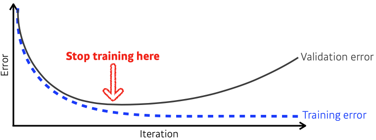
we need additional validation data to do early stopping
-> validation data : train에 활용되지 않는 dataset
cost(error)가 커지는 시점에 stop한다.

Parameter Norm Penalty (Weight Decay)

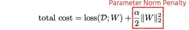
adds smoothness to the function space → 부드러운 함수일수록 generalization performance가 올라갈 것이라 가정
NN parameters가 너무 커지지 않게 제약을 건다 → weight decay
L2 Regularization, L1 Regularization이 존재한다.
Reference
https://deepapple.tistory.com/6
https://huidea.tistory.com/154

Data Augmentation

More data are always wecomed

Noise Robustness

add random noises inputs or weights → data augmentation은 input data만 추가
왜 잘되는지는 아직까지 의문

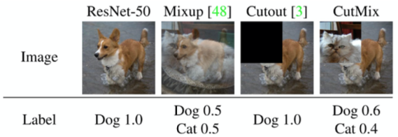
Label Smoothing

≈ Data Augmentation
constructs augmented training exaples by mixing both input and output of two randomly selected training data

Dropout

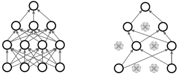
NN train 시 (forward/backward propagation) dropout ratio만큼 각 layer의 neuron을 0으로 바꾸어준다.
각각의 neuron이 좀 더 robust한 feature를 잡을 수 있다; voting 효과 (증명 X)
Reference
https://algopoolja.tistory.com/50

Batch Normalization

compute the empirical mean and variance independently for each dimension (layers) and normalize
-> 각 layer의 statistic을 정규화

$\mu_B = \frac1m \sum^m_{i=1}x_i$
$\sigma^2_B = \frac1m \sum^m_{i=1}\left(x_i - \mu_B\right)^2$
$\hat{x}_i = \frac{x_i - \mu_B}{\sqrt{\sigma^2_B + \epsilon}}$
→ 평균을 빼고 표준편차로 나눠준다.

different variances of normalizations

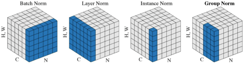
- Batch norm : layer 전체를 줄임
- Layer norm : 각 layer 정보를 줄임
- Instance norm : 데이터 별로 줄임

Image Reference

William JO

🏆

이전 포스트

[2주차] 8.9 월

다음 포스트

[2주차] 8.10 화

Naver Boostcamp AI Tech 2기

✏️Optimization

Optimization이란?

Generalization(일반화)

Underfitting vs. Overfitting

Cross-validation(K-fold validation)

Bias and Variance

Bias and Variance Tradeoff

Bootstrapping (Ensemble)

Reference

✏️Practical Gradient Descent Methods

Gradient Descent Methods

Batch-size Matters

Gradient Descent

Momentum

Nesterov Accelerated Gradient(NAG)

Adagrad

Adadelta

RMSprop

Adam(Adaptive Moment Estimation)

Reference

✏️Regularization

Early Stopping

Parameter Norm Penalty (Weight Decay)

Data Augmentation

Noise Robustness

Label Smoothing

Dropout

Batch Normalization

Image Reference

[2주차] 8.9 월

[2주차] 8.11 수

0개의 댓글

관련 채용 정보