✏️Convolutional Neural Networks(CNN)

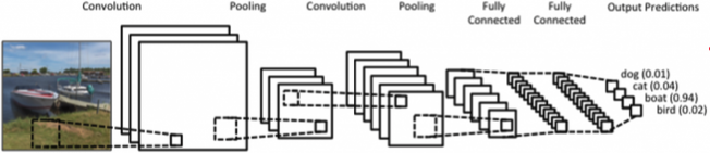
• CNN consists of convolution layer, pooling layer and fully connected layer(FC layer).
• Convolution and pooling layer : feature extraction(정보 추출)
• Fully connected layer : decision making(e.g. classification)
• 최근 FC layer를 없애거나 최소화 시키는 추세 (# parameters ⬆)
  -> 학습 어렵고 generalization performance ⬇(학습 모델이 실제 data에서 얼마나 잘 동작하는지)
• FC layer 대신 convolutional layer로 대체 (conv layer # parameters <<< dense layer # parameters)
  -> convolution layer의 kernel이 모든 위치에 동일하게 적용되기 때문
  (convolution operator = shared parameter)

Convolution

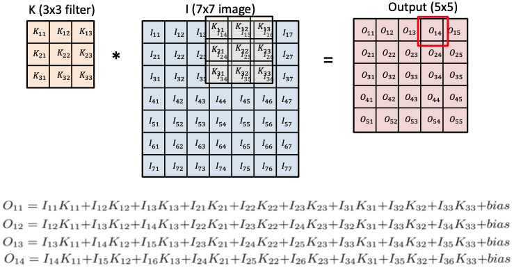
• filter = kernel
• receptive field(국부 수용영역): filter가 한 번에 보는 영역의 크기; 입력의 spatial dimension

RGB Image Convolution

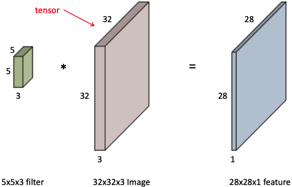
• input image channel size = filter(kernel) channel size

output width = $\frac{width - filter width + (2\times padding)}{stride} + 1$
output height = $\frac{height - filter height + (2\times padding)}{stride} + 1$

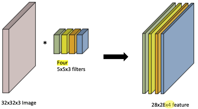
• convolutional feature map의 channel size = filter(kernel) 개수

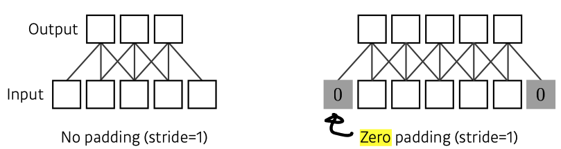
Padding

• boundary(edge) information을 keep하기 위해
  

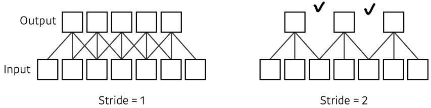
Stride

Convolution Arithmetic (# parameters 계산)

• padding과 stride는 parameter 계산과 무관하다.
• kernel width x kernel height x # input channel x # output channel + # output channel bias
  
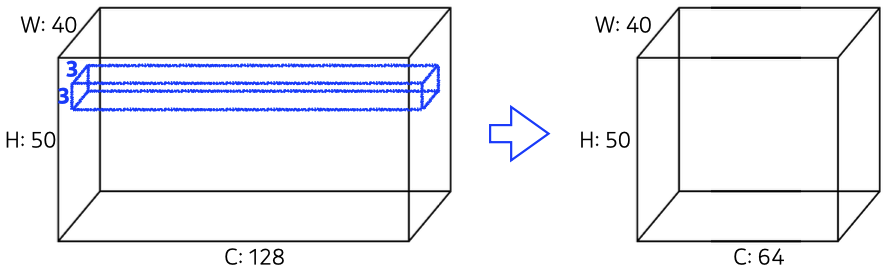
  ex) # params = 3 x 3 x 128 x 64 + 64 = 73,792

1 x 1 Convolution (중요)

• image의 한 pixel만 보는 것; spatial dimension은 유지, channel만 줄임.
• Dimension(channel) reduction
• to reduce the # parameters while increasing the depth (e.g. bottleneck architecture)
  -> FC layer는 # parameters가 많기 때문에, conv layer를 깊게 쌓고 # parameters를 줄이는 것이 좋다.

---

✏️CNN history

• 핵심 : network depth는 점점 깊어지지만, # parameters가 줄어들며 performance가 올라가는 모델들이 나왔다.
  -> 하지만 최근 GPT-3나 dall-e처럼 데이터가 많으면 # parameters가 많아지는 건 당연한듯

ILSVRC

• ImageNet Large-Scale Visual Recognition Challenge
• Classification / Detection / Localization / Segmentation
• 1,000 different categories (classification task)
• Over 1 million images
• Training set : 456,567 images

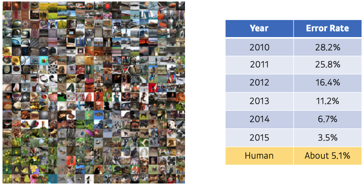
• 2015년 이후로는 error rate 계산의 의미가 없음.

AlexNet

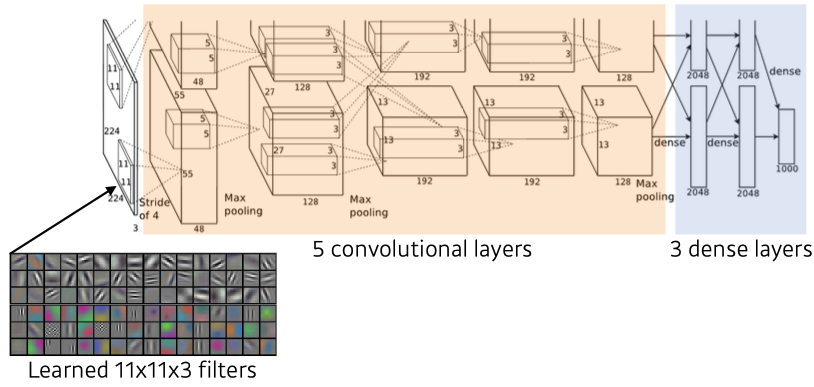
• 최초로 Deep Learning Architecture를 이용하여 ILSVRC에서 수상.
• ReLU activation
  -> preserves good properties of linear models
  -> easy to optimize with gradient descent
  -> overcome the vanishing gradient problem
  -> good generalization
• 2 GPUs implementation
• Local response normalization, Overlapping pooling
• Data augmentation
• Dropout

VGGNet

• 3x3 Convolution을 이용하여 Receptive field는 유지하면서 더 깊은 네트워크를 구성.
• increasing depth with 3x3 convolution filters (with stride 1)
  
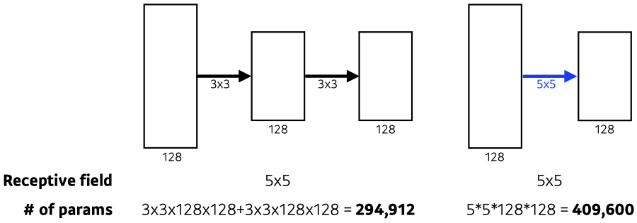
  -> # parameters ⬇, 마지막 convolutional feature map이 보는 receptive field는 같다!
• 1x1 convolution for fully connected layers
• Dropout(p=0.5)

GoogLeNet

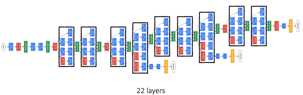
• combined network-in-network(NiN) with inception blocks
  
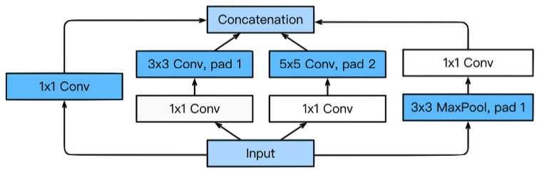
• Inception blocks
  • 하나의 입력이 여러 개로 퍼졌다가 하나로 concat.
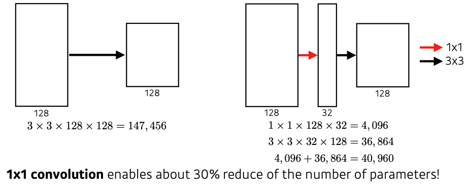
  • reduce the number of parameter → 1x1 convolution as channel-wise dimension reduction
• Benefit of 1x1 convolution
  
  

ResNet

• h(x) = f(x) + x의 구조
• performance increases while parameter size decreases.
• residual connection(= skip connection = identity map)이라는 구조를 제안.
  
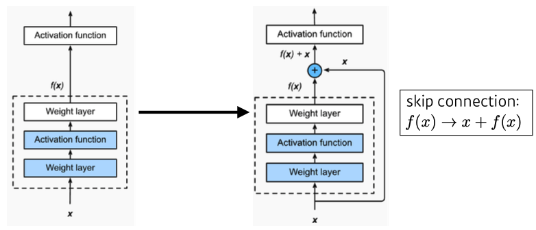
  • conv layer가 학습하는 quantity는 'residual(잔차,차이)'만 학습한다.
  • 깊게 쌓아도 학습 가능!
    
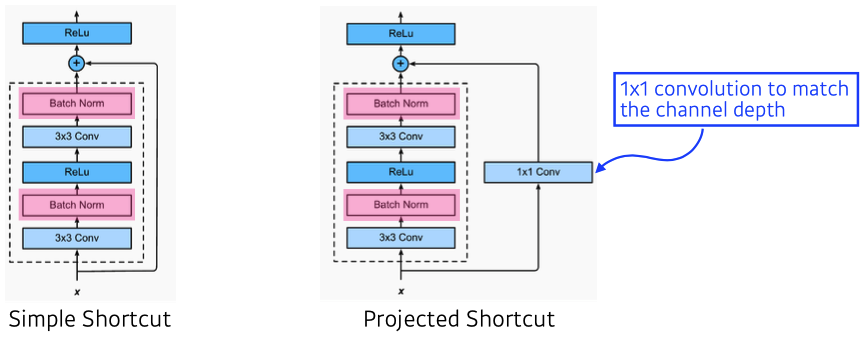
  • 일반적으로 simple shortcut을 씀
  • ReLU와 BN 순서에 대해 논란이 많다. (논문에서는 위 처럼 구조)
• Bottleneck architecture
  
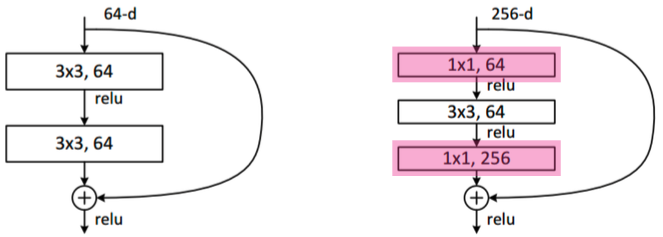
  • GoogLeNet의 inception blocks와 유사

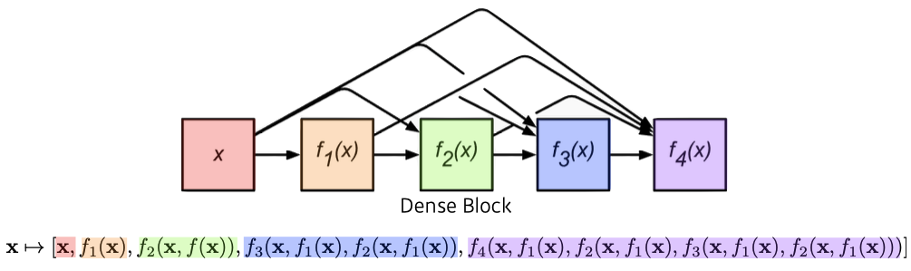
DenseNet

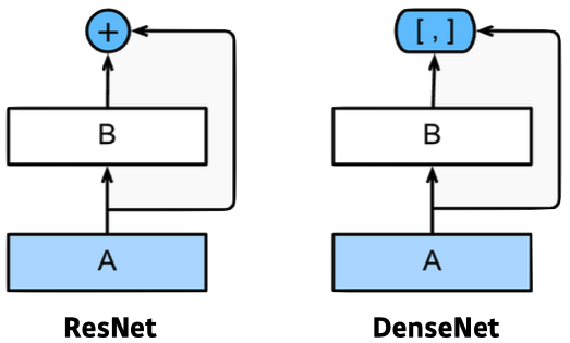
• ResNet과 비슷한 아이디어지만 Addition이 아닌 Concatenation을 적용한 CNN
  • 정보가 섞이기 때문
  • But, channel이 기하급수적으로 커짐 → 뒤로 갈수록 앞 값을 다 concat하기 때문 (# parameters ⬆)
    

Summary

1. VGG : repeated 3x3 blocks → # parameters ⬇, receptive field 유지
2. GoogLeNet : 1x1 convolution → channel-wise dimension reduction
3. ResNet : skip-connection → network depth ⬆
4. DenseNet : concatenation → performance ⬆ than addition(ResNet)

---

✏️Computer Vision Applications

Semantic Segmentation (= Dense Classification)

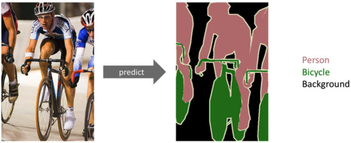
• 각 이미지의 pixel마다 분류 (자율주행, 운전보조장치 쪽에 많이 쓰임)

Fully Convolutional Network

• Vanilla CNN
  
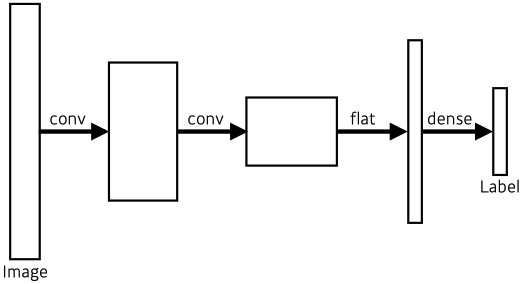
• Fully Convolutional Network
  
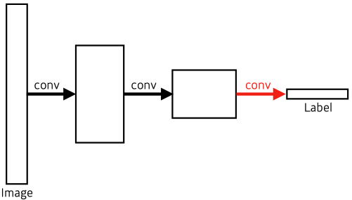
  • No dense layer → convolutionalization
  • # parameters are same between dense layer and FC network
    
    

Convolutionalization

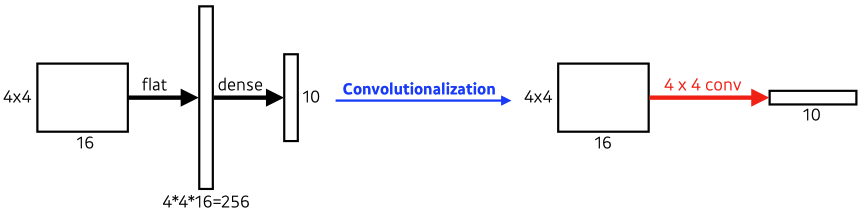
• # parameters (left) : 4 x 4 x 16 x 10 = 2560
• # parameters (right) : 4 x 4 x 16 x 10 = 2560
  
  

Why should you use Fully Convolutional Network?

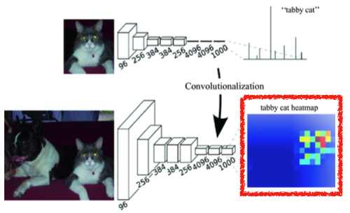
1. Transforming fully connected layers into convolution layers enables a classification net to output a heat map
-> spatial information(위치 정보)를 유지
2. FC(Dense) layer는 fixed input size를 갖지만, FC network는 convolution 연산이 갖는 shared parameter 성질로 input spatial dimensions에 independent하다.

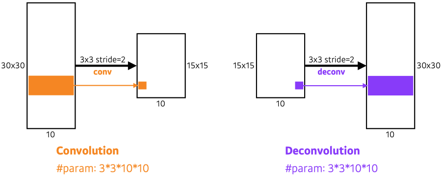
Upsampling

• While FCN can run with input of any size(spatial dimensions) the output dimensions are typically reduced by subsampling. ex) 100x100 → 10x10
• we need a way to connect the coarse output to the dense pixels. →upsampling 기법
  
  

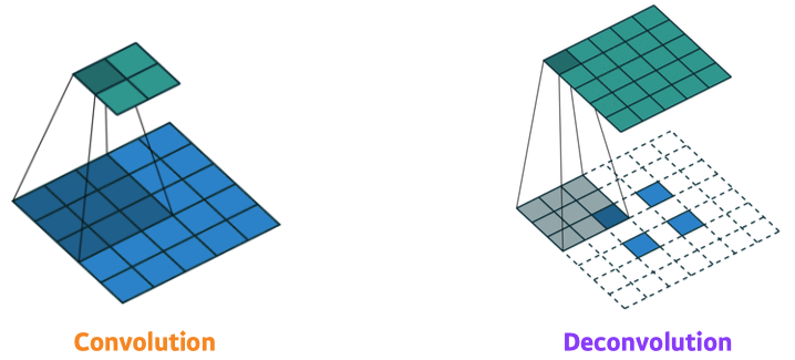
1. Deconvolution(conv transpose)
   • backward convolution (convolution 역연산)
   • 완전 복원은 불가능 → 10 = 3+7 = 2+8 = ...
     
     
     
     

Reference

• https://hugrypiggykim.com/2019/09/29/upsampling-unpooling-deconvolution-transposed-convolution/
• https://kuklife.tistory.com/117
• https://m.blog.naver.com/laonple/220958109081

Detection

• semantic segmentation : per pixel ↔ detection : bounding box (patch)
  
  

R-CNN

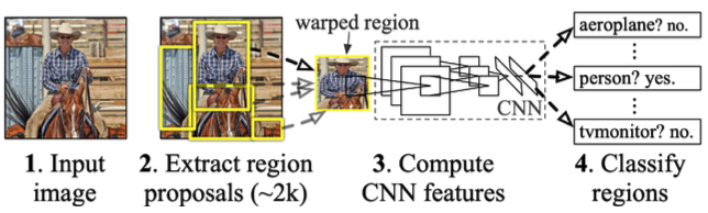
1. takes an input image
2. extracts around 2,000 region proposals (etracts patches randomly) → Selective search
3. compute features for each proposal using AlexNet
4. classfies with linear SVMs

• 굉장히 brute force 스럽고 오래 걸린다.
  
  

SPPNet

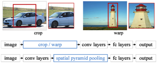
• In R-CNN, CNN must run more than 2,000 times → 각각의 patch마다 CNN 돌려야 함
• In SPPNet, CNN runs once
• input image를 CNN에 넣어 feature map을 뽑고, 그 feature map에서 bounding box마다 값을 뽑아 낸다.
  
  

Fast R-CNN

1. takes an input and a set of bounding boxes → using selective search
2. gnerated convolutional feature map → SPPNet과 동일
3. For each region, get a fixed length feature from ROI(Region of Interest) pooling
4. Two outputs : class and bounding-box regressor

• SPPNet과 거의 유사하지만 NN으로 다 처리
  
  

Faster R-CNN

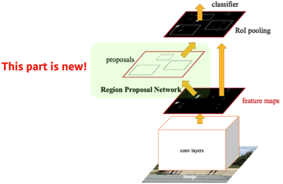
• Fast R-CNN + Region Proposal Network
• selective search는 임의로 bounding-box를 뽑지만, bounding-box candidate 설정 법도 NN으로 학습하자
• Region Proposal Network
  
  • Region Proposal : 특정 영역(patch)이 bounding-box로서 의미가 있을지(target이 있을지) 찾아준다.
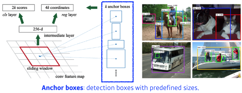
  • Anchor boxes : detection boxes with predefined sizes(template); 미리 정한 bounding-box 크기
    

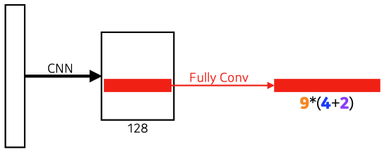
    9 : Three different region sizes (128, 256, 512) with three different ratios (1:1, 1:2, 2:1)
          →3 x 3 = 9, anchor boxes
    4 : four bounding box regression parameters
    2 : box classification (whether to use it or not) → yes or no

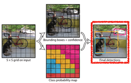
YOLO (You Only Look Once)

• YOLO(v1) is an extremely fast object detection algorithm

• ⭐️ It simultaneously predicts multiple bounding boxes and class probabilities

  • bounding box를 따로 뽑아서 분류하지 않고, 한번에 진행

• No explicit bounding box sampling (compared with Faster R-CNN)

  • Region Proposal Network에서 나온 bounding box sub-tensor를 분류하지 않는다.

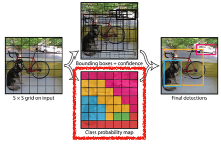
• Given an image, YOLO divides it into SxS grid.
  

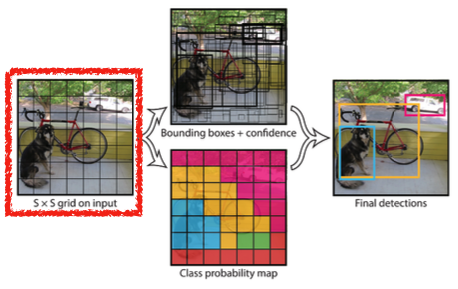
  • if the center of an object falls into the grid cell, that grid cell is responsible for detection.
  • detection target center가 해당 grid 안에 있으면 그 grid cell이 해당 물체에 대한 bounding box, class를 예측

• Each cell predicts B bounding boxes (B=5)
  

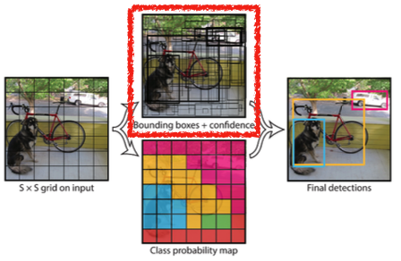
  • Each bounding box predicts
    -> box refinement (x, y, w, h)
    -> confidence (of objectness) → box probability

• Each cell predicts C class probabilities
  

• In total, it becomes a tensor with S x S x (B * 5 + C) size

  • S x S : Number of cells of the grid
  • B * 5 : B bounding boxes with offsets (x, y, w, h) and confidence
    -> B x [x, y, w, h, c]
    
  • C : Number of classes