Classification

1. MNIST

a set of 70,000 small images of digits handwritten by high school students and employees of the US Census Bureau.

often called the “hello world” of Machine Learning

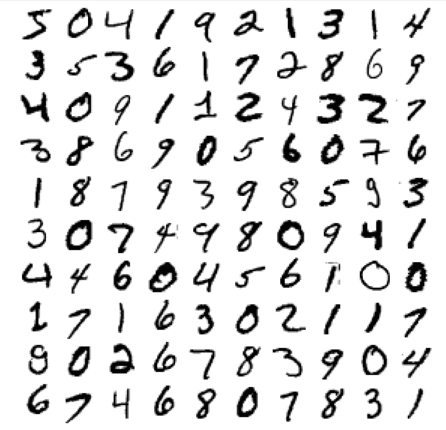
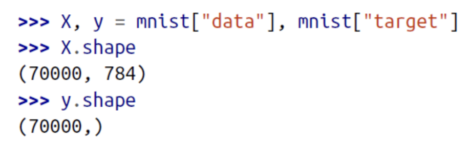
There are 70,000 images, and each image has 784 features.

This is because each image is 28 × 28 pixels, and each feature simply
represents one pixel’s intensity, from 0 (white) to 255 (black).

2. Training a Binary Classifier

Let’s simplify the problem for now and only try to identify one digit

from sklearn.linear_model import SGDClassifier
sgd_clf = SGDClassifier(random_state=42)
sgd_clf.fit(X_train, y_train_5)

3. Performance Measures

Let’s use the cross_val_score() function to evaluate our SGDClassifier model, using K-fold cross-validation with three folds.

>>> from sklearn.model_selection import cross_val_score
>>> cross_val_score(sgd_clf, X_train, y_train_5, cv=3, scoring="accuracy")
array([0.96355, 0.93795, 0.95615])

Let’s look at a very dumb classifier that just classifies every single image in the “not-5” class:

• over 90% accuracy even a dumb classifier.
• This is simply because only about 10% of the images are 5s, so if you always guess that an image is not a 5, you will be right about 90% of the time.

💡 This is why accuracy is generally not the preferred performance measure for classifiers

Confusion Matrix

A much better way to evaluate the performance of a classifier is to look at the confusion matrix.

from sklearn.metrics import confusion_matrix

confusion_matrix(y_train_5, y_train_pred)

array([[53057, 1522],
			 [1325, 4096]])

Precision and Recall

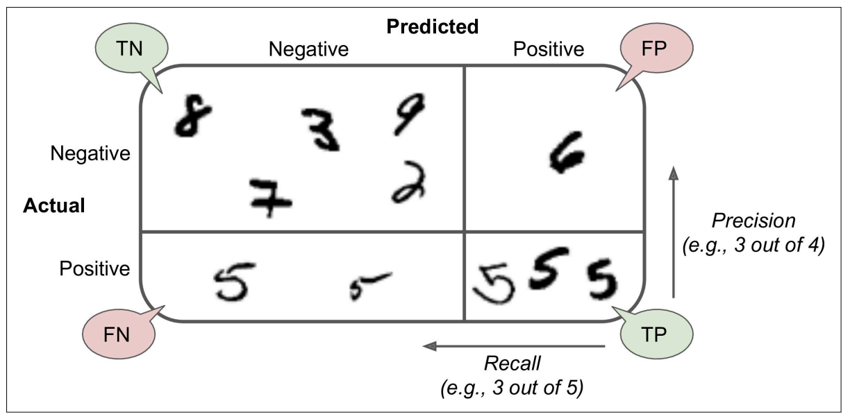
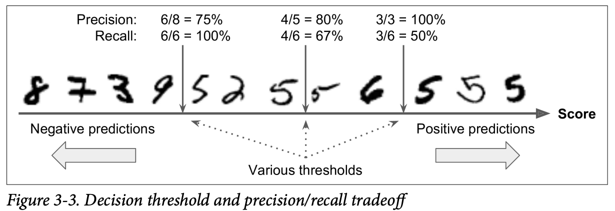
Precision

Recall

from sklearn.metrics import precision_score, recall_score

>>> precision_score(y_train_5, y_train_pred) # == 4096 / (4096 + 1522)
0.7290850836596654
>>> recall_score(y_train_5, y_train_pred) # == 4096 / (4096 + 1325)
0.7555801512636044

When it claims an image represents a 5, it is correct only 72.9% of the time. Moreover, it only detects 75.6% of the 5s.

It is often convenient to combine precision and recall into a single metric called the F1 score.

This is not always what you want: in some contexts you mostly care about precision, and in other contexts you really care about recall.

• Ex1: if you trained a classifier to detect videos that are safe for kids, you would probably prefer a classifier that rejects many good videos (low recall) but keeps only safe ones (high precision), rather than a classifier that has a much higher recall but lets a few really bad videos show up in your product.
• Ex2: Suppose you train a classifier to detect shoplifters in surveillance images: it is probably fine if your classifier has only 30% precision as long as it has 99% recall (sure, the security guards will get a few false alerts, but almost all shoplifters will get caught).

💡 Unfortunately, you can’t have it both ways: increasing precision reduces recall, and vice versa. This is called the precision/recall trade-off.

ROC Curve

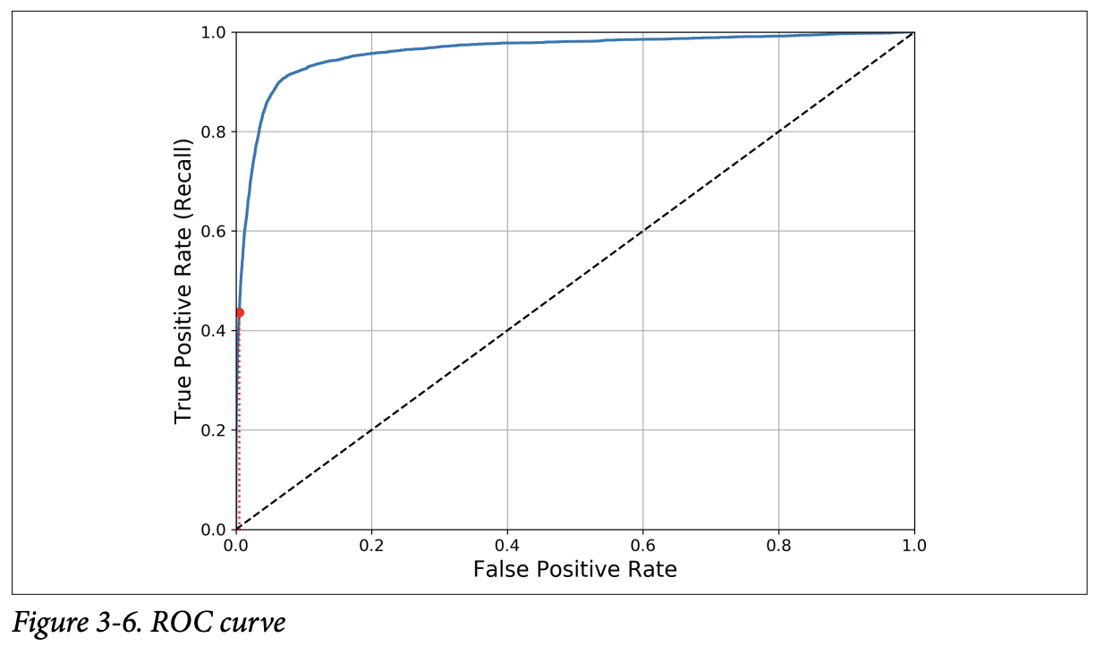
• ROC curve plots the true positive rate (another name for recall) against the false positive rate (FPR).
• Once again there is a trade-off: the higher the recall (TPR), the more false positives (FPR) the classifier produces.
• The dotted line represents the ROC curve of a purely random classifier; a good classifier stays as far away from that line as possible (toward the top-left corner).

4. Multiclass Classification

one-versus-the-rest (OvR) strategy (also called one-versus-all)

• Classify the digit images into 10 classes (from 0 to 9) is to train 10 binary classifiers, one for each digit (a 0-detector, a 1-detector, a 2- detector, and so on).
• Then when you want to classify an image, you get the decision score from each classifier for that image and you select the class whose classifier outputs the highest score

one-versus-one (OvO) strategy

• Train a binary classifier for every pair of digits: one to distinguish 0s and 1s, another to distinguish 0s and 2s, another for 1s and 2s, and so on.
• If there are N classes, you need to train N × (N – 1) / 2 classifiers.
• When you want to classify an image, you have to run the image through all 45 classifiers (for MNIST problem) and see which class wins the most duels.

5. Error Analysis

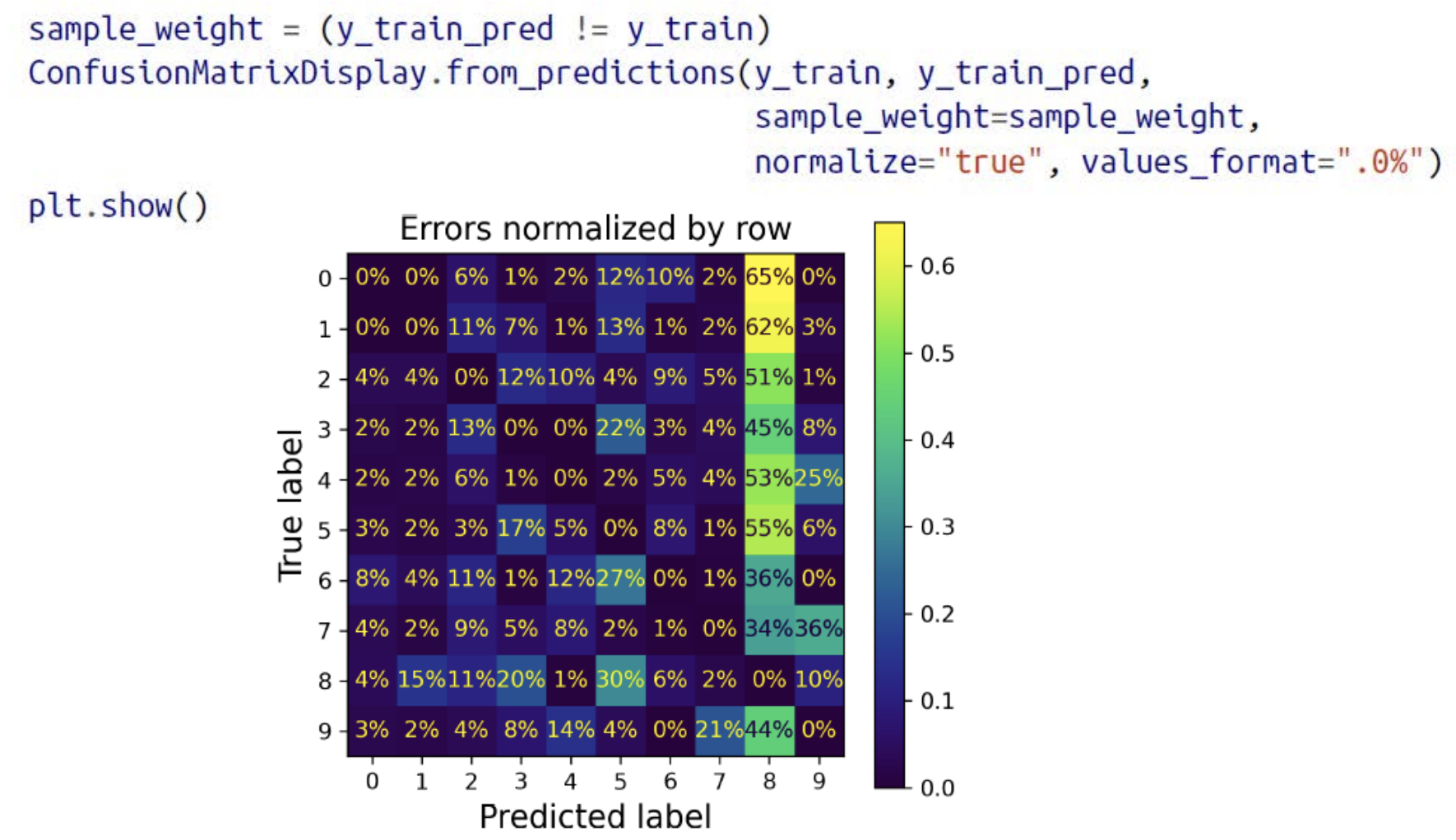
• The column for class 8 is quite bright, which tells you that many images get misclassified as 8s.
• As you can see, the confusion matrix is not necessarily symmetrical. You can also see that 3s and 5s often get confused (in both directions).

6. Multilabel Classification

In some cases you may want your classifier to output multiple classes for each instance.

ex) train classifier(Kneighbors) → measure(F1 score)

If you wish to use a classifier that does not natively support multilabel classification, such as SVC, one possible strategy is to train one model per label.

To solve this issue, the models can be organized in a chain: when a model makes a prediction, it uses the input features plus all the predictions of the models that come before it in the chain

7. Multioutput Classification

Generalization of multilabel classification where each label can be multiclass

i.e., it can have more than two possible values