1. Decision Tree (Training, Visualizing, Making Predictions)

Like SVMs, Decision Trees are versatile Machine Learning algorithms that can perform both classification and regression tasks, and even multioutput tasks.

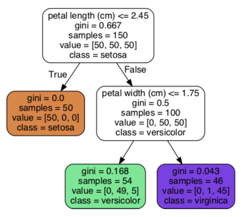
A node’s samples attribute counts how many training instances it applies to.

• Ex: 100 training instances have a petal length greater than 2.45 cm (depth 1, right), and of those 100, 54 have a petal width smaller than 1.75 cm (depth 2, left).

A node’s value attribute tells you how many training instances of each class this node applies to

• Ex: the bottom-right node applies to 0 Iris setosa, 1 Iris versicolor, and 45 Iris virginica

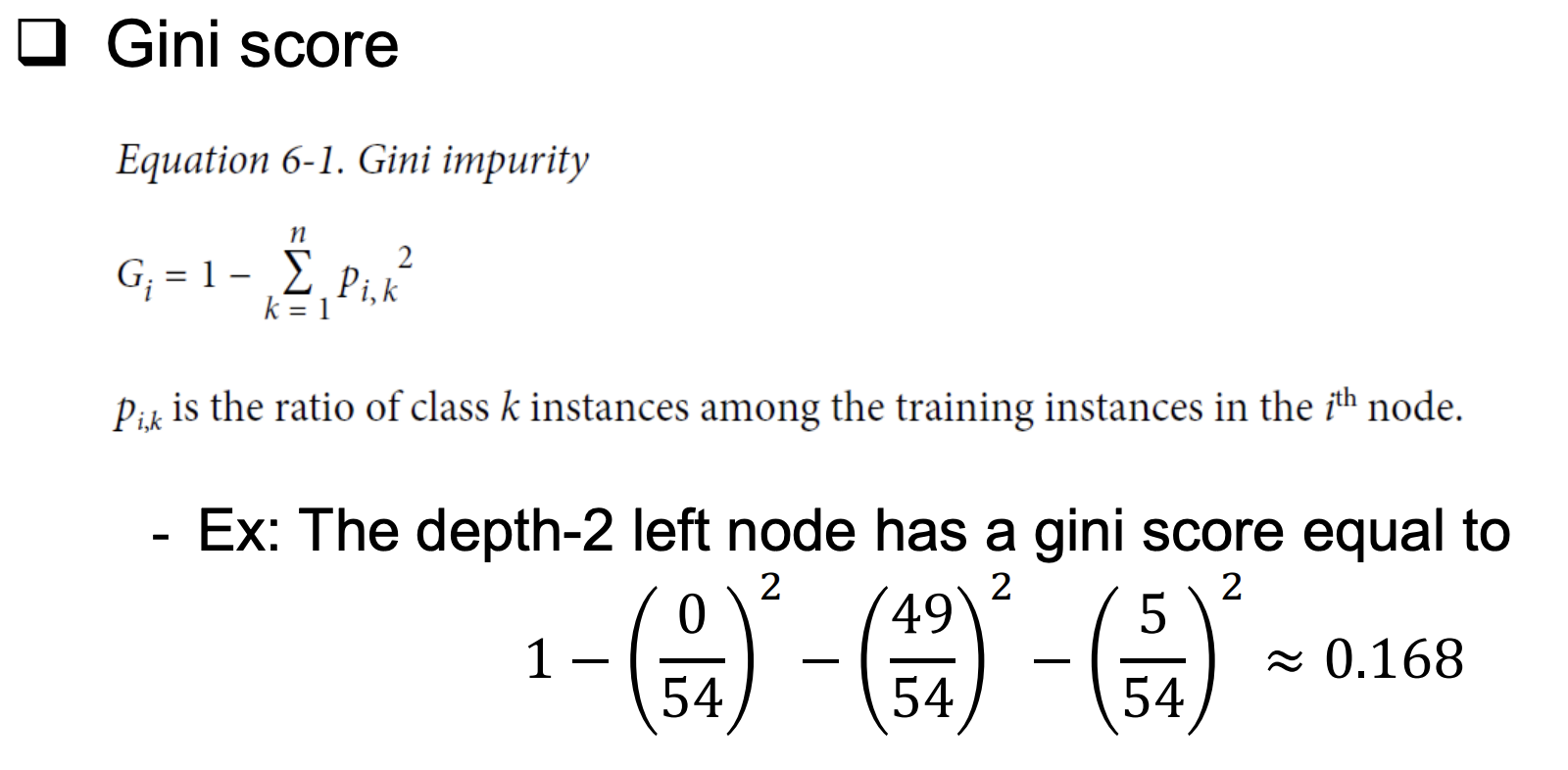
A node’s gini attribute measures its impurity: a node is “pure” (gini=0) if all training instances it applies to belong to the same class.

• EX: since the depth-1 left node applies only to Iris setosa training
  instances, it is pure and its gini score is 0

A Decision Tree can also estimate the probability that an instance belongs to a particular class k. First it traverses the tree to find the leaf node for this instance, and then it returns the ratio of training instances of class k in this node.

• Ex: suppose you have found a flower whose petals are 5 cm long and 1.5 cm wide. The corresponding leaf node is the depth-2 left node, so the Decision Tree should output the following probabilities: 0% for Iris setosa (0/54), 90.7% for Iris versicolor (49/54), and 9.3% for Iris virginica (5/54).

2. The CART Training Algorithm

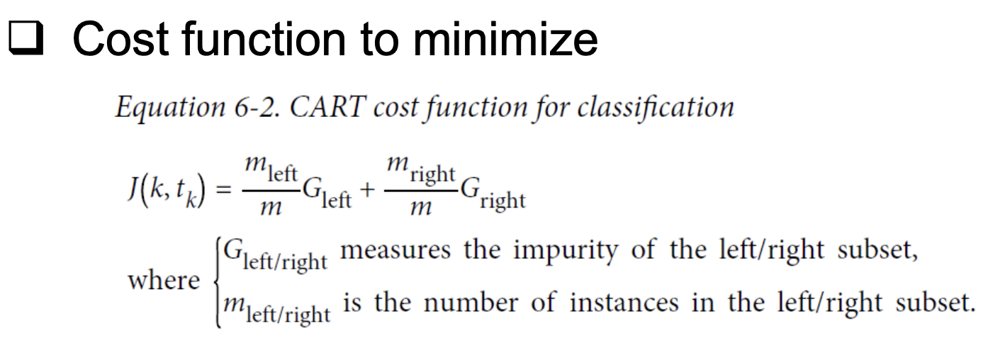
Once the CART algorithm has successfully split the training set in two, it splits the subsets using the same logic, then the sub-subsets, and so on, recursively.

CART algorithm is a greedy algorithm. Unfortunately, finding the optimal tree is known to be an NPComplete problem.

• It requires O(exp(m)) time, making the problem intractable even for small training sets.

3. Regularization Hyperparameters

Decision Trees make very few assumptions about the training data.

• As opposed to linear models, which assume that the data is linear.

If left unconstrained, the tree structure will adapt itself to the training data, fitting it very closely—indeed, most likely overfitting it.

• Such a model is often called a nonparametric model, not because it does not have any parameters but because the number of parameters is not determined prior to training, so the model structure is free to stick closely to the data.

To avoid overfitting the training data, you need to restrict the Decision Tree’s freedom during training. (=regularization)

• You can at least restrict the maximum depth of the Decision Tree.

The DecisionTreeClassifier class has a few other parameters that similarly restrict the shape of the Decision Tree:

• min_samples_split (the minimum number of samples a node must have before it can be split)
• min_samples_leaf (the minimum number of samples a leaf node must have)
• min_weight_fraction_leaf (same as min_samples_leaf but expressed as a fraction of the total number of weighted instances)
• max_leaf_nodes (the maximum number of leaf nodes)
• and max_features (the maximum number of features that are evaluated for splitting at each node).

❑ Increasing min* hyperparameters or reducing max* hyperparameters will regularize the model.

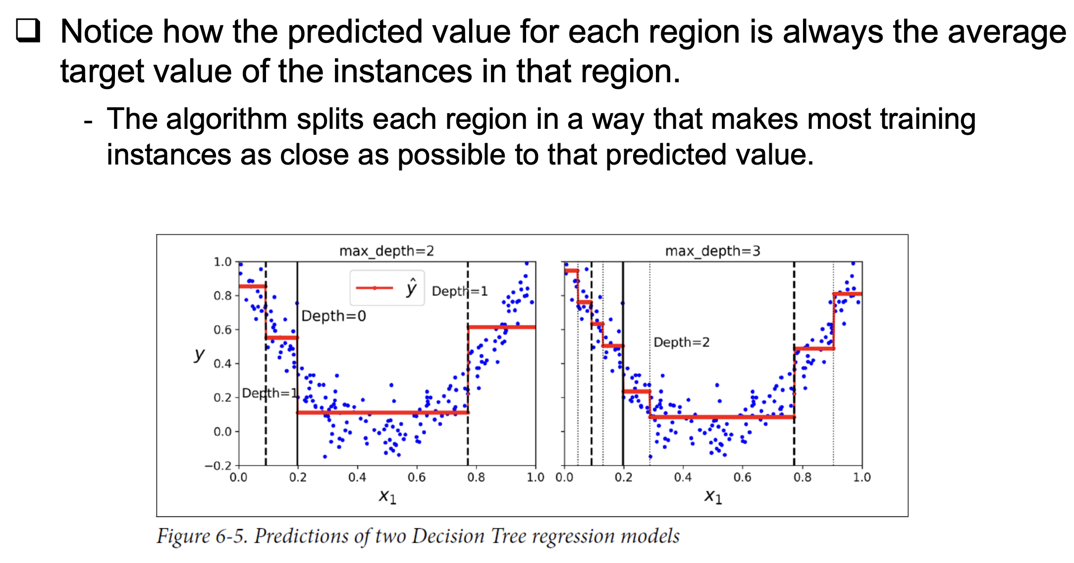
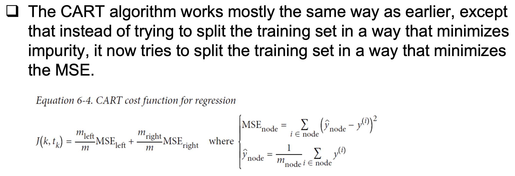
4. Regression

• The main difference is that instead of predicting a class in each node, it predicts a value.
• Ex: x1=0.6, then predicts value =0.111. This prediction is the average target value of the 110 training instances associated with this leaf node, and it results in a mean squared error equal to 0.015 over these 110 instances.

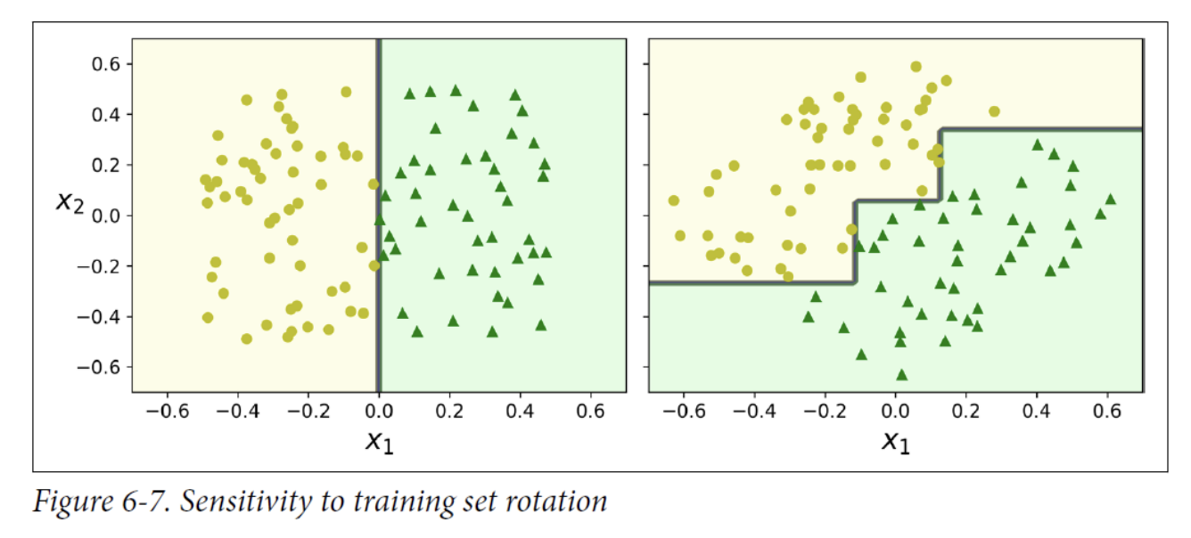
5. Instability

Decision Trees love orthogonal decision boundaries (all splits are perpendicular to an axis), which makes them sensitive to training set rotation.

• On the left, a Decision Tree can split it easily, while on the right, after the dataset is rotated by 45°, the decision boundary looks unnecessarily convoluted.