1. Linear SVM Classification

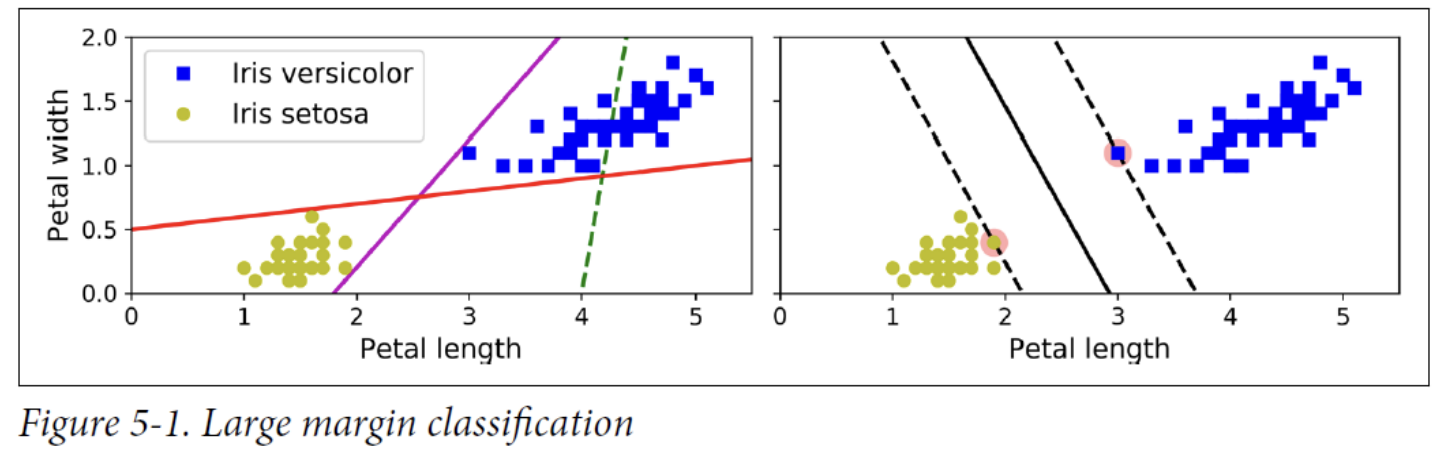
These instances are called the support vectors (SVM decision boundary). They are circled in Figure 5-1.

SVMs are sensitive to the feature scales. -> scaling is necessary!!

Hard margin classification

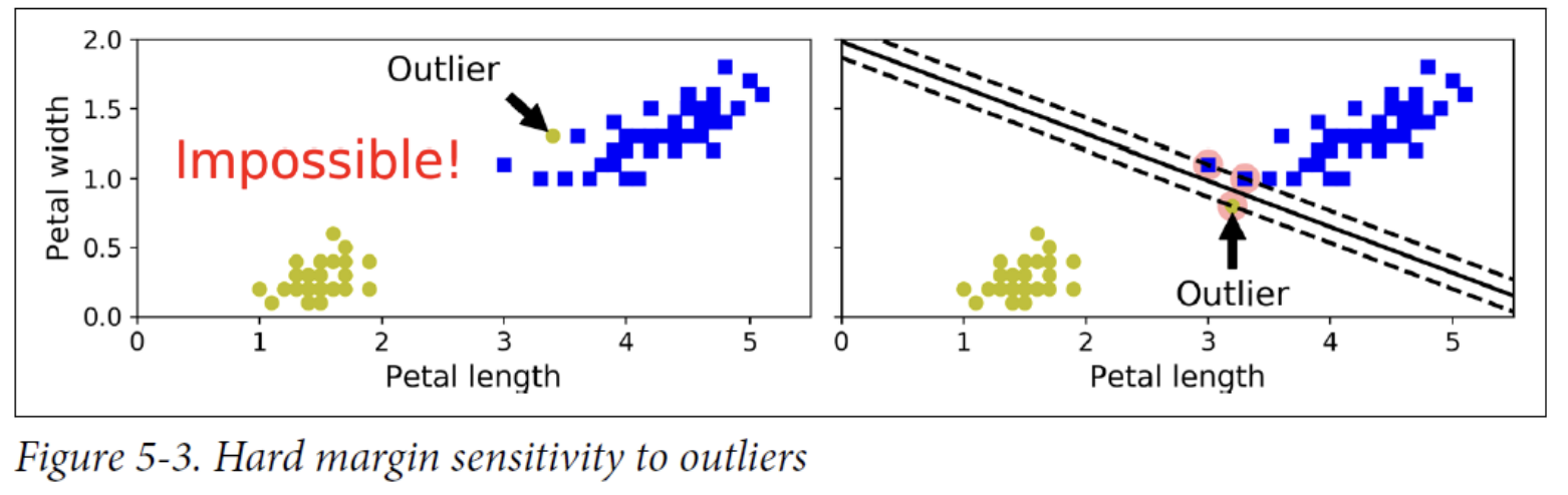
Two main issues with hard margin classification:

• First, it only works if the data is linearly separable.
• Second, it is sensitive to outliers.

Soft margin classification

• To avoid these issues, use a more flexible model.
• The objective is to find a good balance between keeping the street as large as possible and limiting the margin violations (i.e., instances that end up in the middle of the street or even on the wrong side).
  

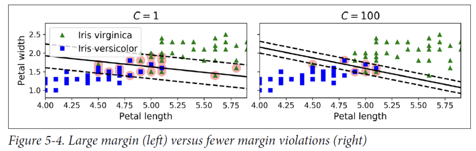
C = 1 margin increase -> violation increase -> flexible -> not overfitting

C = 100 margin decrease -> violation decrease -> train fitting (noise sensitive) -> overfitting

2. Nonlinear SVM Classification

Polynomial Kernel

Fortunately, when using SVMs you can apply an almost miraculous mathematical technique called the kernel trick.The kernel trick makes it possible to get the same result as if you had added many polynomial features, even with very high-degree polynomials, without actually having to add them.

So there is no combinatorial explosion of the number of features because you don’t actually add any features.

If your model is overfitting, reduce the polynomial degree.

• If your model is underfitting, increase the polynomial degree.
• Hyperparameter coef0 controls how much the model is influenced by high-degree polynomials vs. low-degree polynomials.

Similarity features

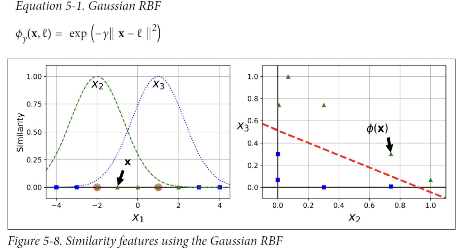
let’s define the similarity function to be the Gaussian Radial Basis Function (RBF) with γ = 0.3. This is a bell-shaped function varying from 0 (very far away from the landmark) to 1 (at the landmark).

How to select the landmarks?

• The simplest approach is to create a landmark at the location of each and every instance in the dataset.
  training data x feature = 100 x 100
• Doing that creates many dimensions and thus increases the chances that the transformed training set will be linearly separable.
• The downside is that a training set with m instances and n features gets transformed into a training set with m instances and m features (assuming you drop the original features).
• If your training set is very large, you end up with an equally large number of features.

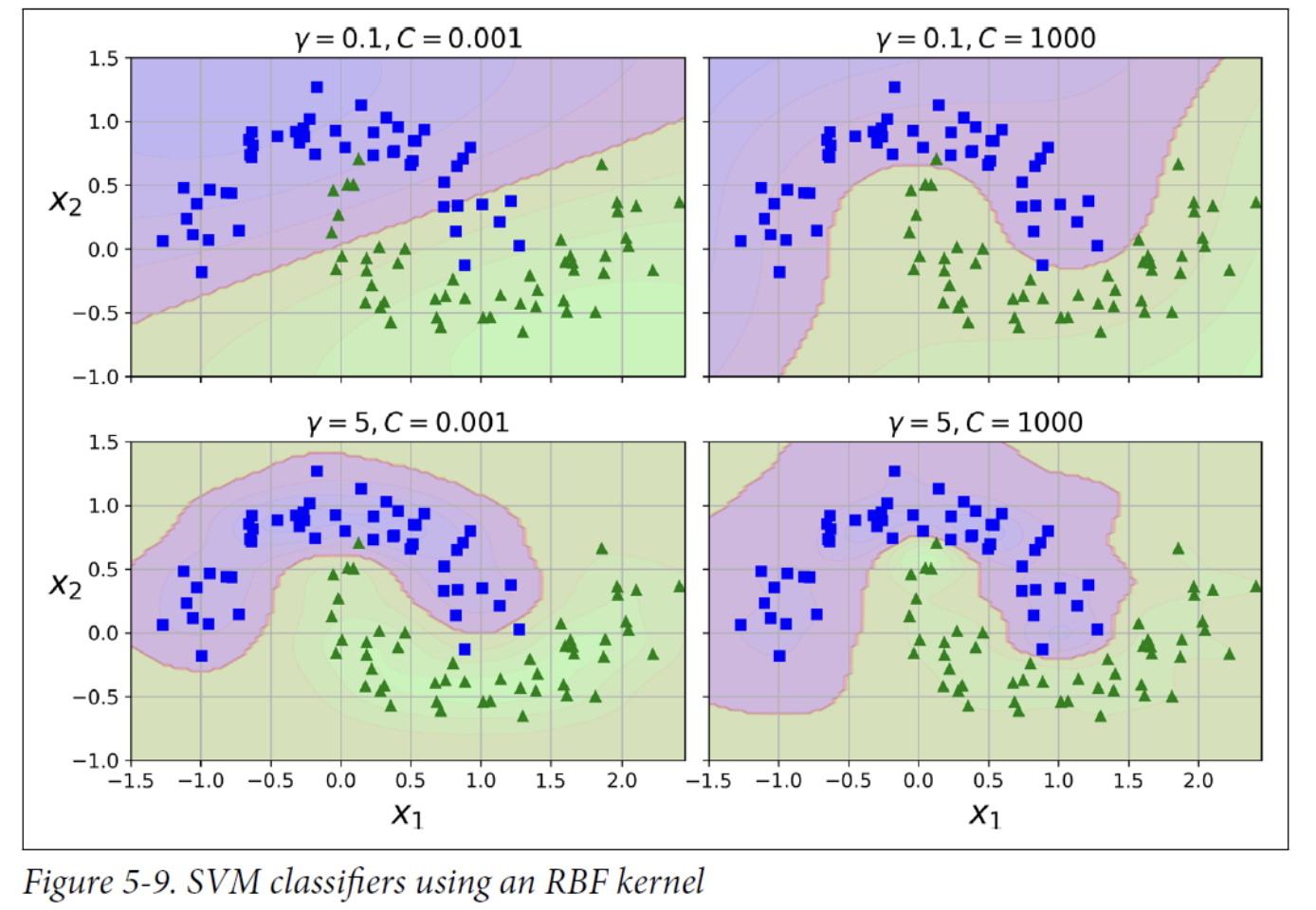
Gaussian RBF Kernel

Hyperparameter 𝛾

• Increasing 𝛾 makes bell-shaped curve narrower, so each instance’s range of influence is smaller: the decision boundary ends up being more irregular, wiggling around individual instances. → possibly overfitting
• Decreasing 𝛾 makes bell-shaped curve wider, so each instance has a larger range of influence: the decision boundary ends up smoother. → possibly underfitting

How to choose the kernel?

• As a rule of thumb, you should always try the linear kernel first, especially if the training set is very large or if it has plenty of features.
• If the training set is not too large, you should also try the Gaussian RBF kernel; it works well in most cases.
• Then if you have spare time and computing power, you can experiment with a few other kernels, using cross-validation and grid search.

The LinearSVC class is based on the liblinear library.

• It does not support the kernel trick, but it scales almost linearly with the number of training instances and the number of features. - O(m × n)
  The SVC class is based on the libsvm library, which implements an algorithm that supports the kernel trick.
• The training time complexity is between 𝑂𝑂(𝑚^2 × 𝑛) and 𝑂(𝑚^3 × 𝑛)
• This means that it gets dreadfully slow when the number of training instances gets large.
• This algorithm is perfect for complex small or medium-sized training sets.

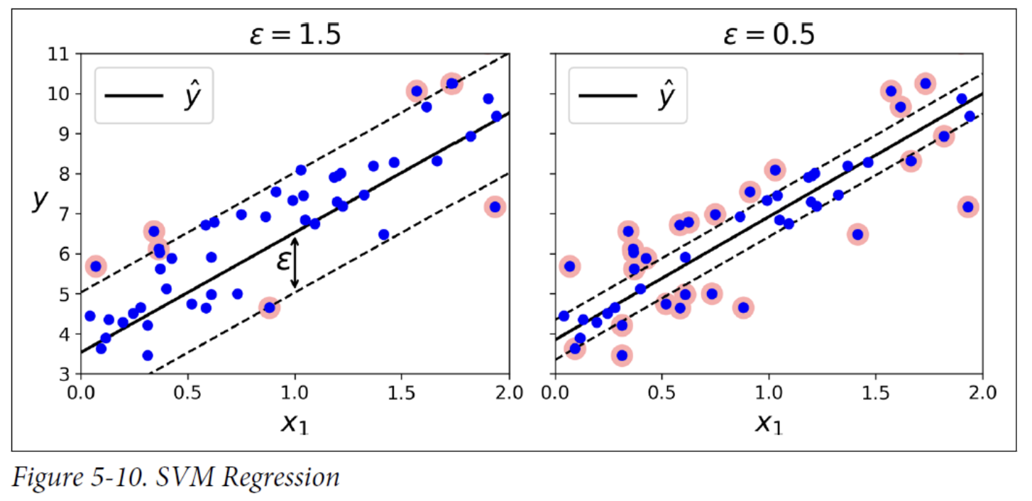
3. SVM Regression

SVM supports linear and nonlinear regression. To use SVMs for regression instead of classification, the trick is to reverse the objective. SVM Regression tries to fit as many instances as possible on the street while limiting margin violations (i.e., instances off the street). The width of the street is controlled by a hyperparameter, 𝜖.

Adding more training instances within the margin does not affect the model’s predictions; thus, the model is said to be ϵ-insensitive.

4. Under the Hood

Hard Margin Objective

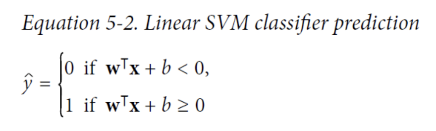
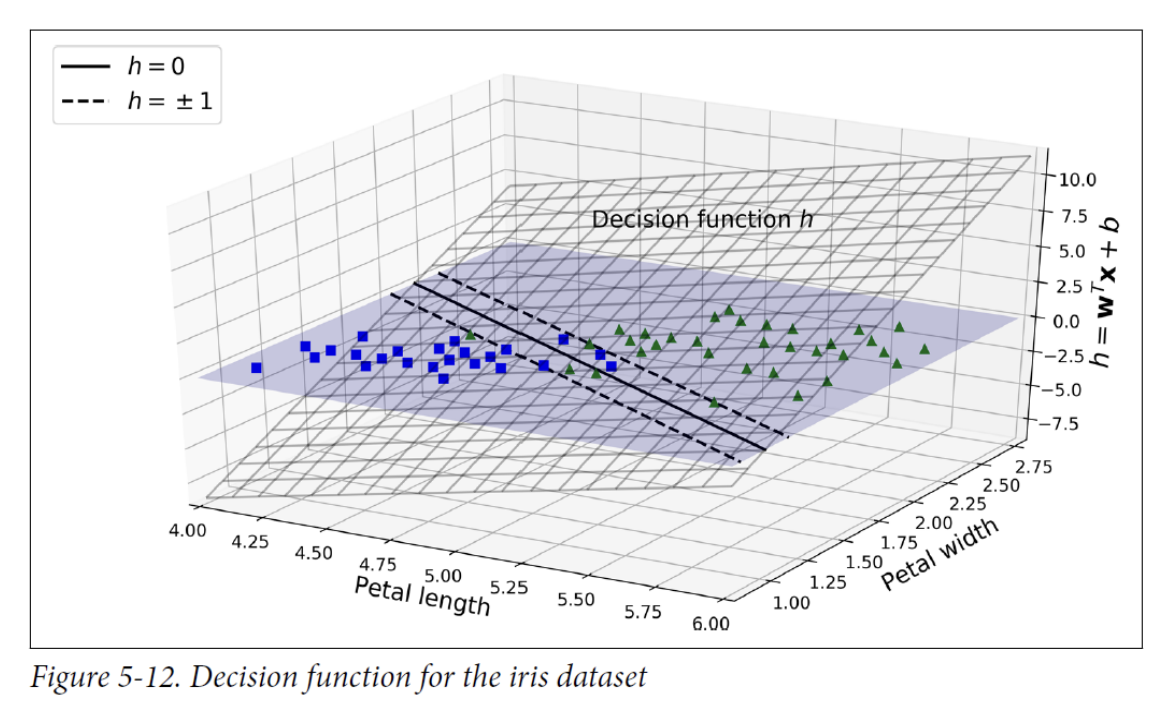
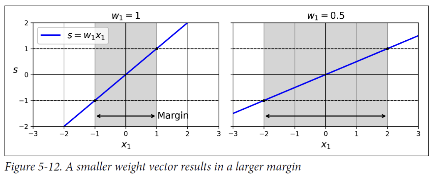
1. we want to minimize | 𝐰 | to get a large margin.
2. If we want to avoid any margin violations (hard margin), then we need the decision function to be greater than 1 for all positive training instances and lower than -1 for negative training instances.

Soft Margin Objective

We now have two conflicting objectives
1. make the slack variables as small as possible to reduce the margin violations.
2. 𝐰𝐓𝐰 as small as possible to increase the margin.
-> This is where C hyperparameter comes in: it allows us to define the trade-off between these two objectives

The hard margin and soft margin problems are both convex quadratic optimization problems with linear constraints. Such problems are known as Quadratic Programming (QP) problems.

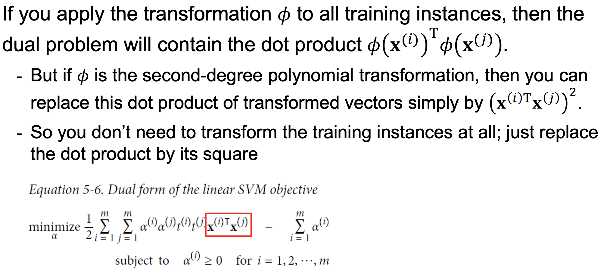
The dual problem

Given a constrained optimization problem, known as the primal problem, it is possible to express a different but closely related problem, called its dual problem.

• Under some conditions, the dual problem can have the same solution as the primal problem
• Condition: the objective function is convex, and the inequality constraints are continuously differentiable and convex functions

Luckily, the SVM problem happens to meet these conditions, so you can choose to solve the primal problem or the dual problem; both will have the same solution.

The dual problem makes the kernel trick possible, while the primal does not.