RNN
시퀀스 데이터
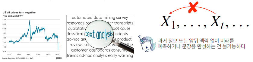
소리, 문자열, 주가 등의 데이터를 시퀀스(sequence) 데이터로 분류
-
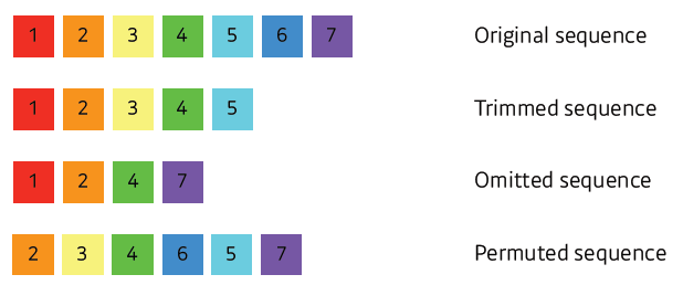
시퀀스 데이터는 독립동등분포(i.i.d.) 가정을 잘 위배하기 때문에 순서를 바꾸거나 과거 정보에 손실이 발생하면 데이터의 확률분포도 바뀌게 됩니다.
-
시계열(time-series) 데이터는 시간 순서에 따라 나열된 데이터로 시퀀스 데이터에 속한다.
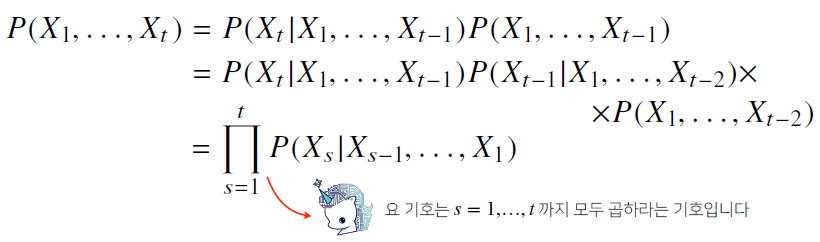
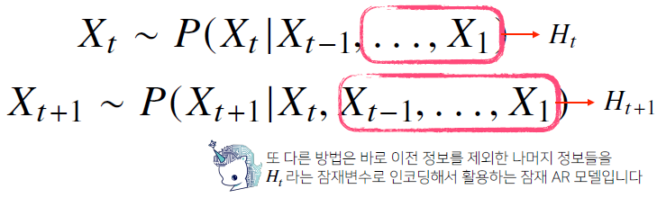
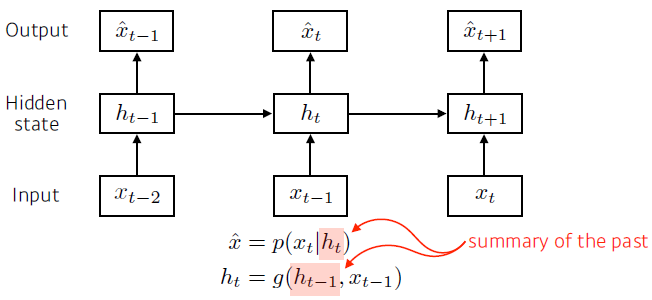
- 이전 시퀀스의 정보를 가지고 앞으로 발생할 데이터의 확률분포를 다루기 위해 조건부확률을 이용할 수 있습니다.
-
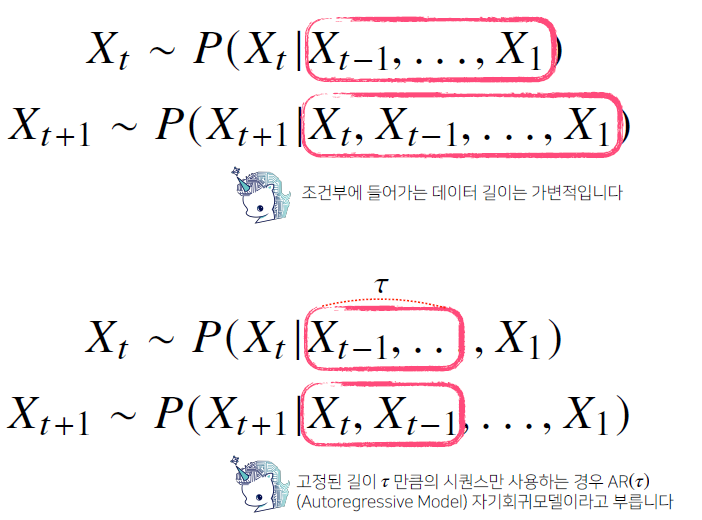
위 조건부확률은 과거의 모든 정보를 사용하지만 시퀀스 데이터를
분석할 때 모든 과거 정보들이 필요한 것은 아닙니다. -
시퀀스 데이터를 다루기 위해선 길이가 가변적인 데이터를 다룰 수 있는 모델이 필요합니다.
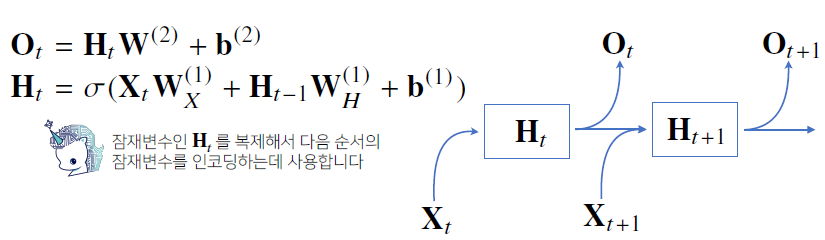
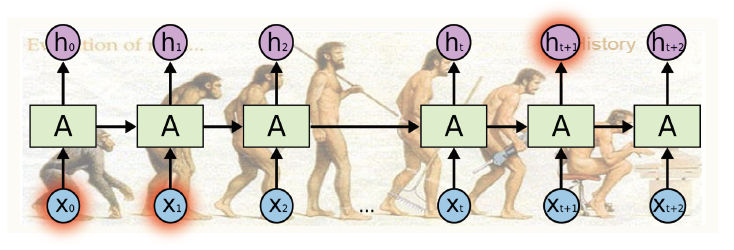
Recurrent Neural Network
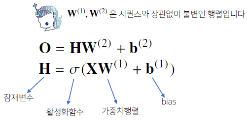
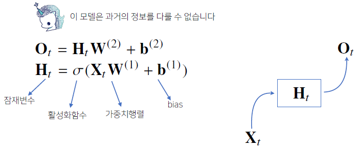
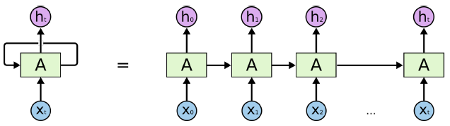
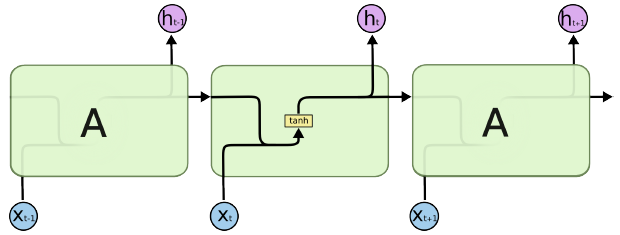
- 가장 기본적인 RNN 모형은 MLP 와 유사한 모양입니다.
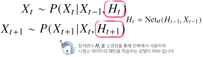
- RNN 은 이전 순서의 잠재변수와 현재의 입력을 활용하여 모델링합니다.
-
여기서 사용되는 가중치인 , , 는 t에 따라서 변하지 않는다. t에 따라서 변하는 것은 오직 잠재변수인 와 입력 데이터인 이다.
-
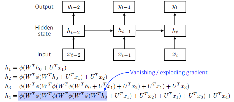
RNN 의 역전파는 잠재변수의 연결그래프에 따라 순차적으로 계산합니다.
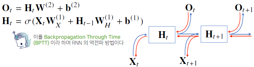
BPTT
- BPTT를 통해 RNN의 가중치행렬의 미분을 계산해보면 아래와 같이
미분의 곱으로 이루어진 항이 계산됩니다.
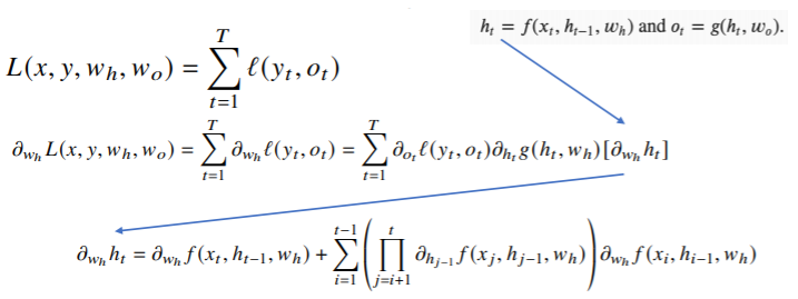
-
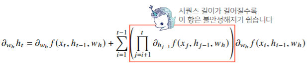
빨간색 항 안의 성분의 크기가 1을 넘으면 gradient 값이 너무 커지게 되고(발산), 크기가 1보다 작으면 gradient vanishing이 일어나게 된다.
-
시퀀스 길이가 길어지는 경우 BPTT 를 통한 역전파 알고리즘의 계산이 불안정 해지므로 길이를 끊는 것이 필요합니다. 이를 truncated BPTT 라 부릅니다. 이런 문제들 때문에 vanilla RNN 은 길이가 긴 시퀀스를 처리하는데 문제가 있습니다. 이를 해결하기 위해 등장한 RNN 네트워크가 LSTM 과 GRU 입니다.
Recurrent Neural Networks
Sequential Model
- Naive sequence model
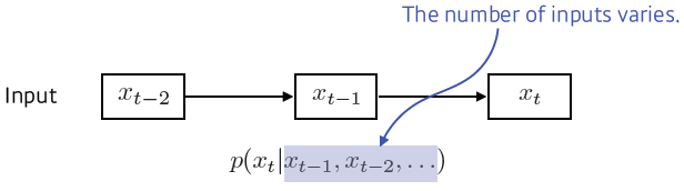
- Autoregressive model
-
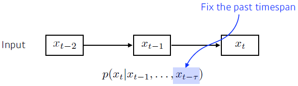
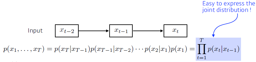
Markov model (first-order autoregressive model)
한계점: 수능 점수가 바로 전날 공부에만 영향을 받지는 않는다.
-
Latent autoregressive model
Recurrent Neural Network
-
Short-term dependencies
인접한 과거의 데이터는 잘 반영한다.
-
Long-term dependencies
먼 과거의 데이터는 잘 반영하지 못 한다.
-
activation function으로 sigmoid를 쓸 경우 정보가 -1 ~ 1 사이로 계속 압축되어 Vanishing gradient 이 발생하고, ReLU를 쓸 때, 정보의 크기가 1보다 큰 경우 Exploding gradient 가 발생한다.
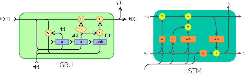
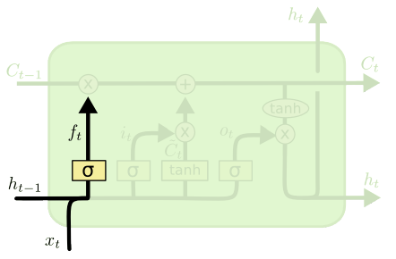
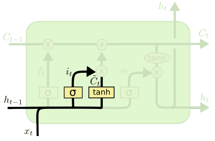
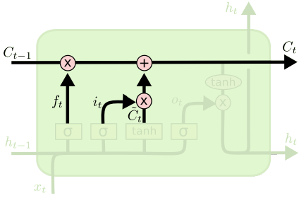
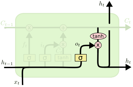
Long Short Term Memory
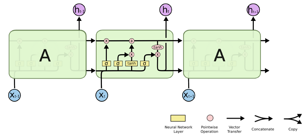
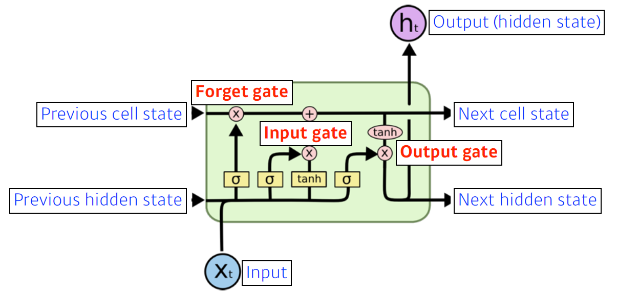
Core idea
cell state (time step t까지의 정보를 요약) 가 지나가면서 어떤 정보가 중요하고 그렇지 않은지 각 gate를 지나며 조작된다.
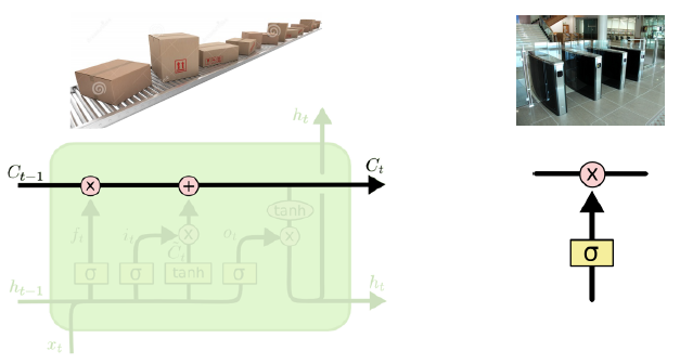
Forget Gate
Decide which information to throw away.
Input Gate
Decide which information to store in the cell state.
Update cell
Update the cell state.
Output Gate
Make output using the updated cell state.
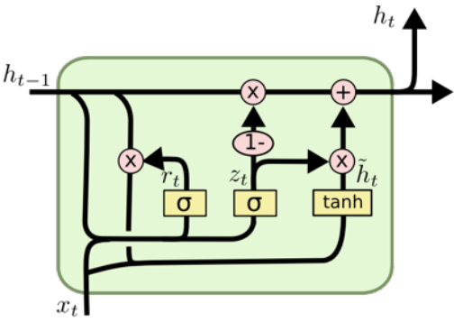
Gated Recurrent Unit
Simpler architecture with two gates (reset gate and update gate).
No cell state, just hidden state.
Transformer
Sequential Model
What makes sequential modeling a hard problem to handle?
Transformer
Transformer is the first sequence transduction model based entirely on attention.
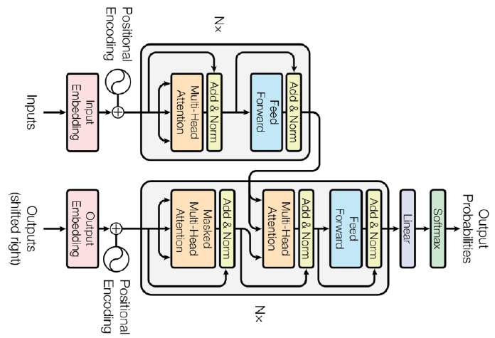
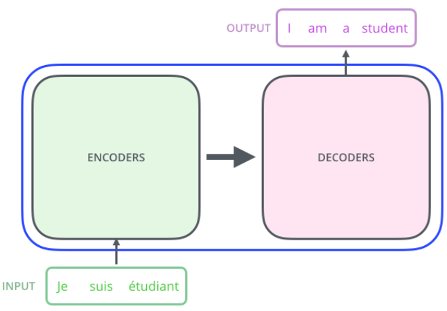
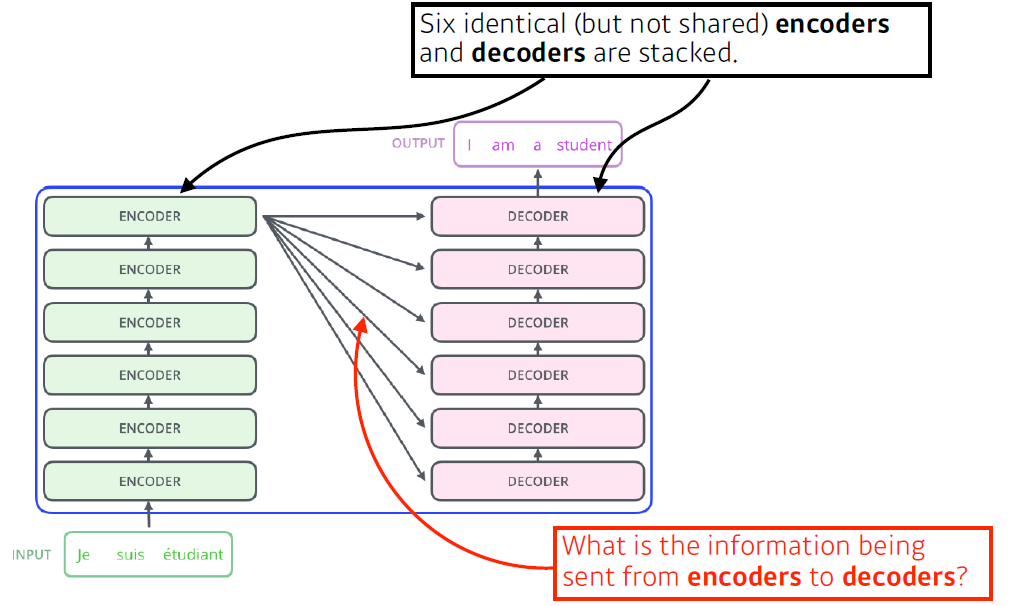
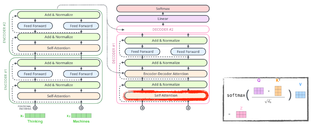
The Self-Attention in both encoder and decoder is the cornerstone of Transformer.
-
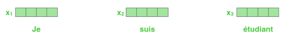
First, we represent each word with some embedding vectors
-
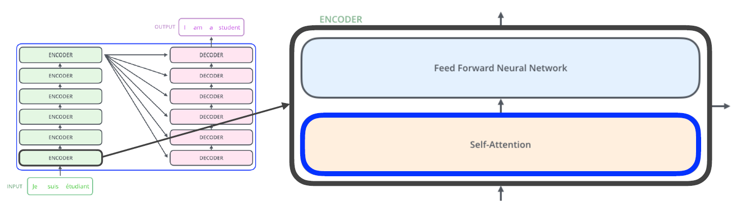
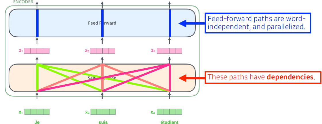
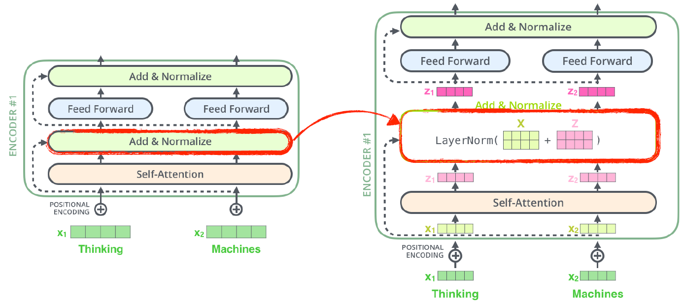
Then, Transformer encodes each word to feature vectors with Self-Attention.
- Self-Attention에서 벡터가 벡터로 될 때 모든 벡터들이 서로 영향을 준다.
- Feed Forward에서는 서로 영향이 없다.
-
Self-Attention at a high level
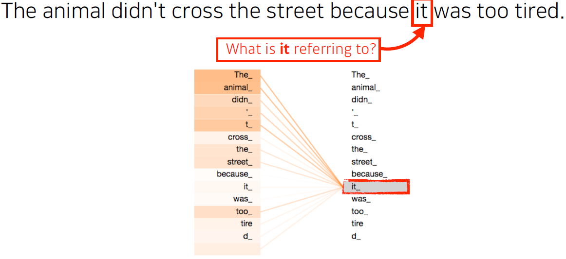
The animal didn't cross the street because it was too tired.-
위 문장을 이해하려고 하면 it이 어떤 단어에 의존하는지 알아야한다. 즉, 하나의 문장에 있는 단어를 설명하려면 단어를 그 자체로 이해하는게 아니라 그 단어가 문장 속에서 다른 단어들과 어떤 관계가 있는지 이해해야 한다.
-
-
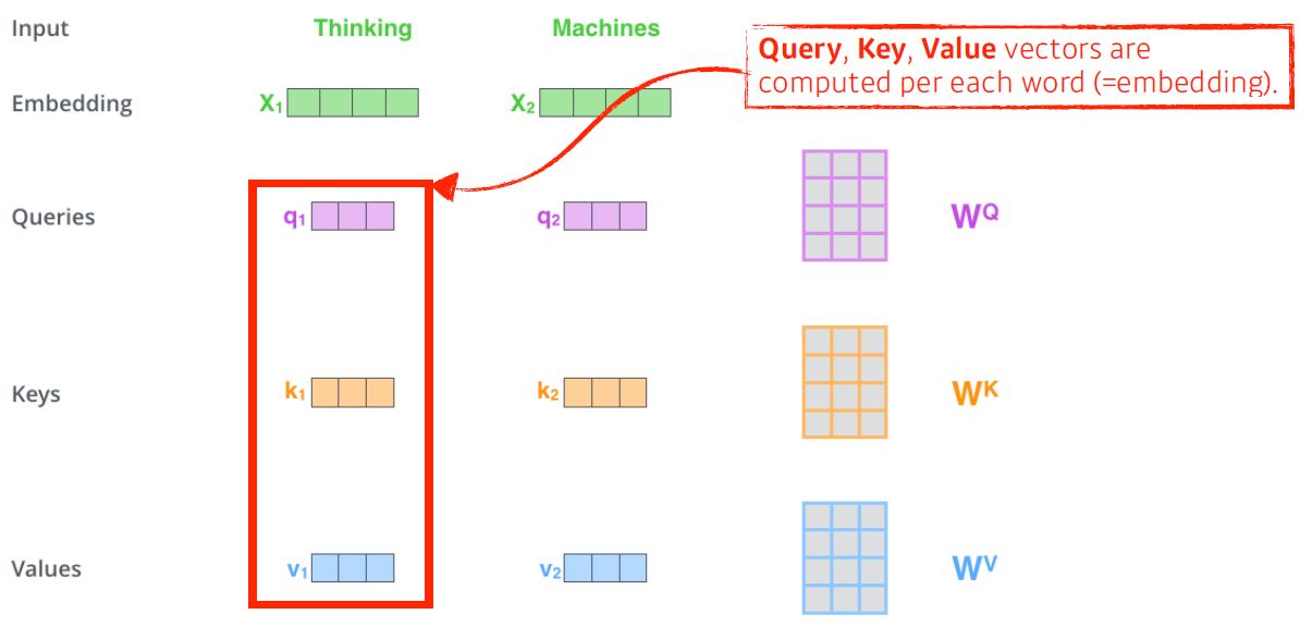
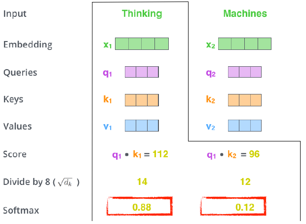
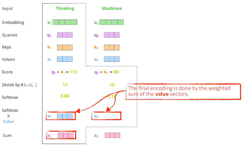
Thinking Machine이라는 단어가 주어지면 각 단어마다 Query, Key, Value 세 벡터가 만들어진다. 이 세 벡터를 통해 임베딩 벡터가 새로운 벡터로 바뀐다.
-
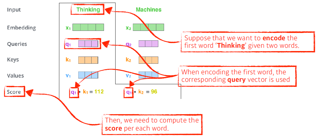
각 단어에 대한 Score 벡터를 계산할 때, encoding을 하고자 하는 Query 벡터()와 나머지 모든 n개의 단어에 대한 Key벡터를 내적을 한다.(Query 벡터와 Key 벡터의 차원이 항상 같아야 한다) i번째 단어가 나머지 n개의 단어와 얼마나 상호작용을 해야하는지 확인해서 학습한다. 이를 Attention이라고 한다. (task를 수행할 때 특정 time step의 입력이 어떤 입력들과 상호관계가 있는지 확인)
-
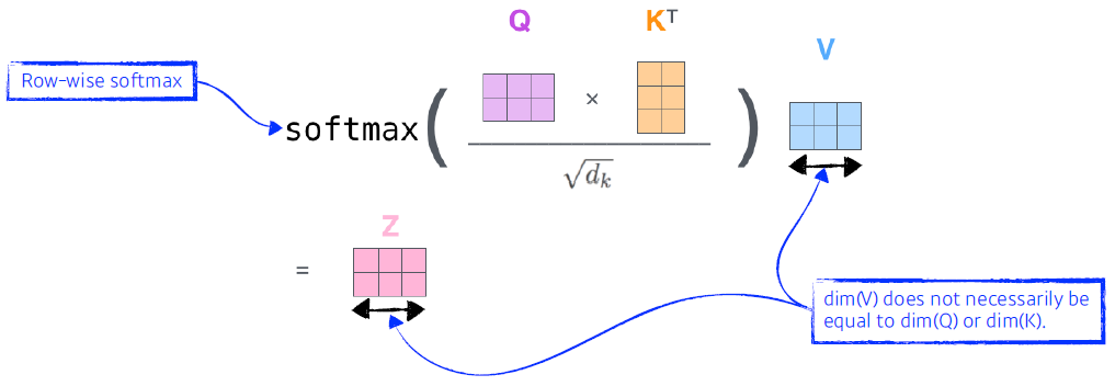
Then, we compute the attention weights by scaling followed by softmax. (아래 그림의 Divide 를 8로 해주는 건 key 혹은 Query 벡터의 차원에 비례한다??)
-
Query 벡터와 Key 벡터는 서로 내적을 하기 때문에 차원이 항상 같아야 한다.
-
벡터의 차원은 벡터의 차원과 같다.
-
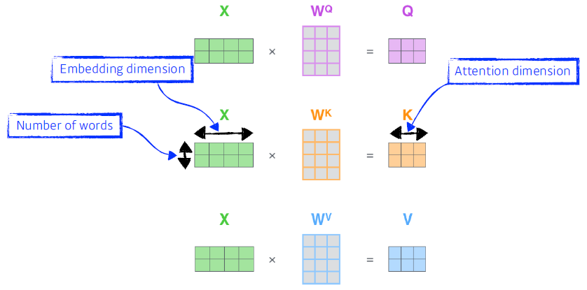
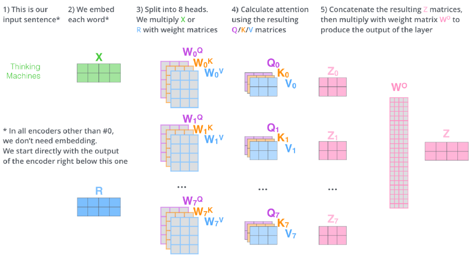
Calculating Q, K, and V from X in a matrix form.
-
입력이 고정되더라도 다른 입력들이 달라지면 출력이 달라진다.(MLP나 FCN과 다르다)
-
Transformer는 N x N 크기의 Attention map을 만든다. (계산량이 많다.)
-
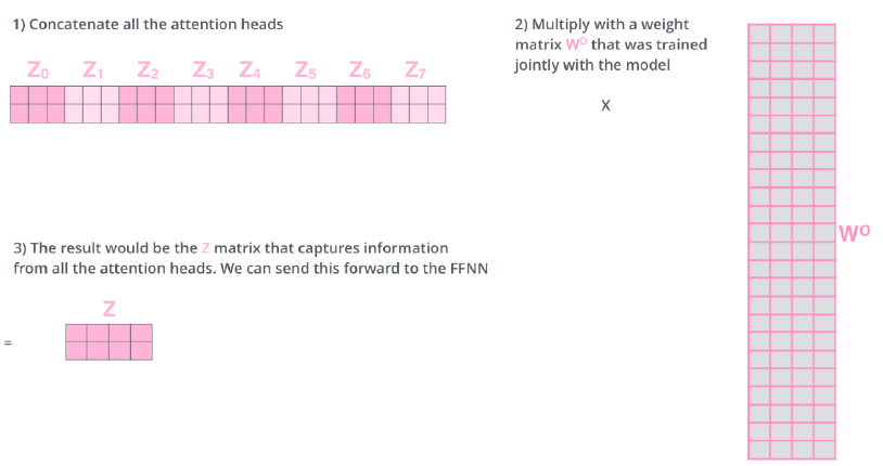
Multi-headed attention (MHA) allows Transformer to focus on different positions. If eight heads are used, we end up getting eight different sets of encoded vectors. (attention heads) MHA는 벡터를 여러개 만든다.
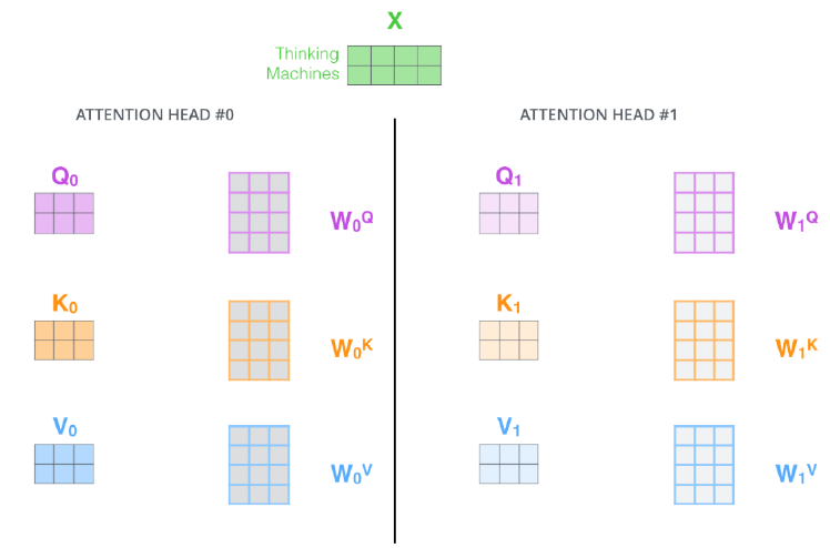
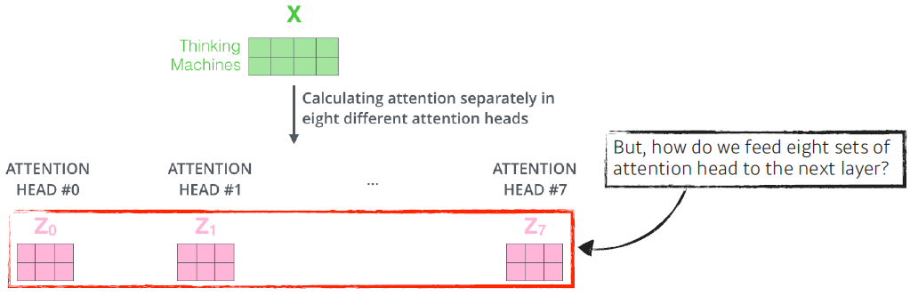
- If eight heads are used, we end up getting eight different sets of encoded vectors (attention heads). We simply pass them through additional (learnable) linear map.
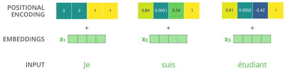
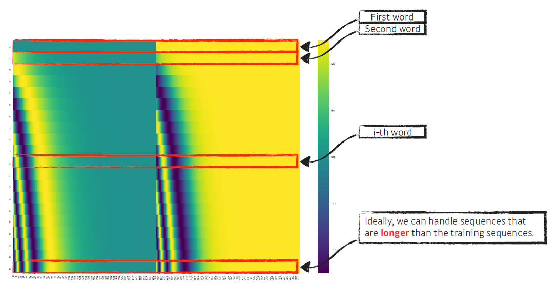
- We need positional encoding. Why?
단어가 (a, b, c, d) 의 순서로 들어가거나, (a, c, b, d)의 순서로 들어가거나 a의 입력에 대한 출력 값이 같아서, 이에 대한 정보를 표시해준다.
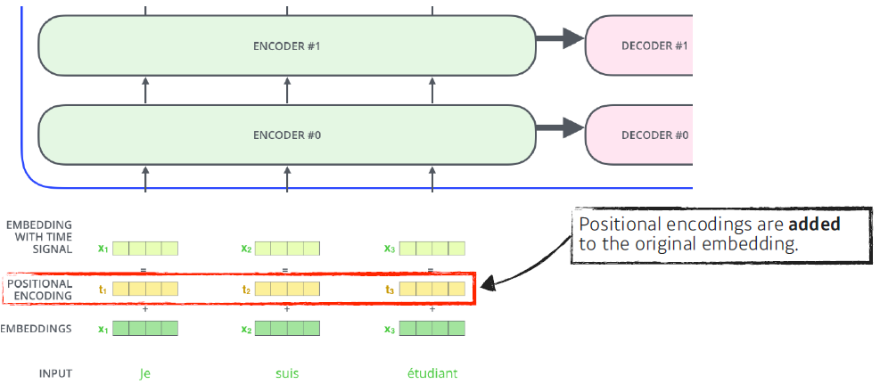
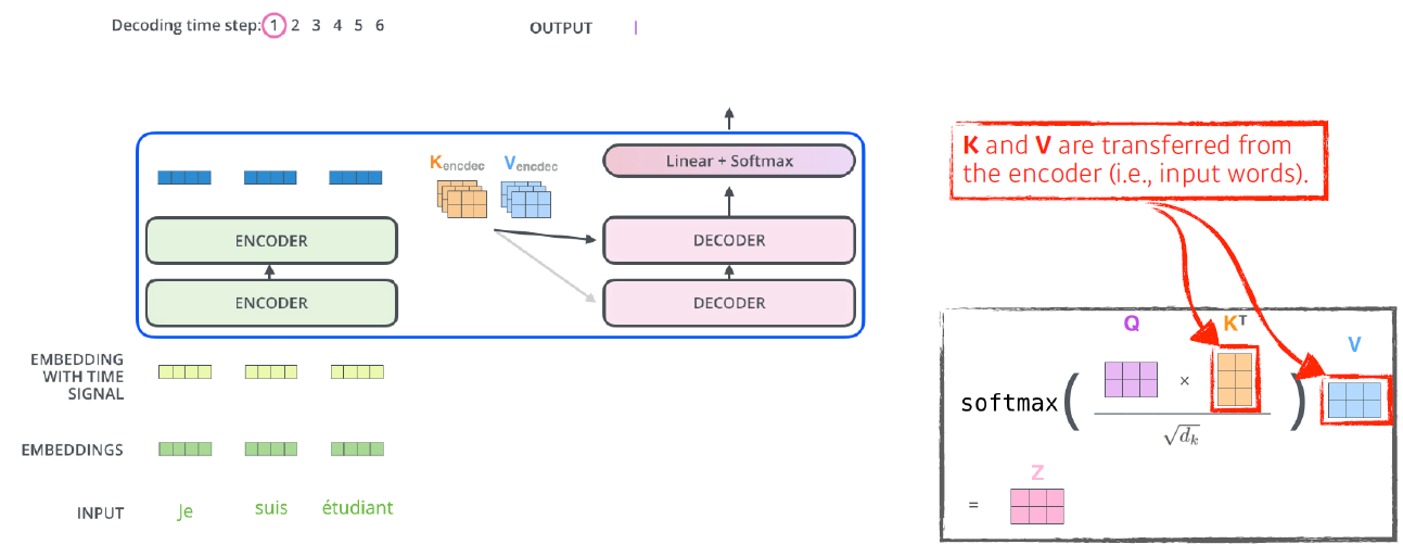
- encoding 된 정보(Key, Value)는 decoder로 보내진다.
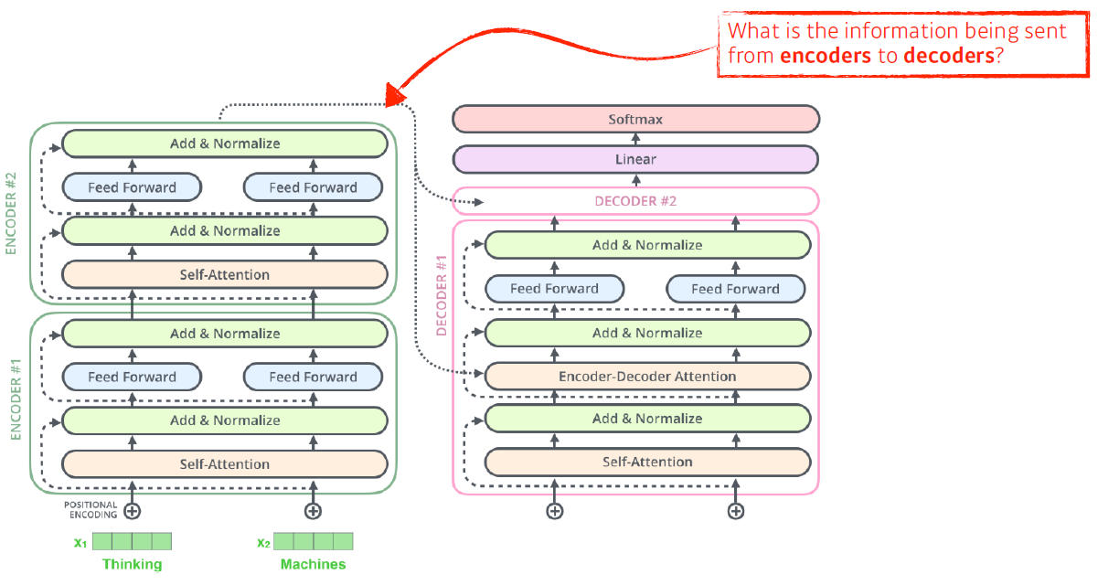
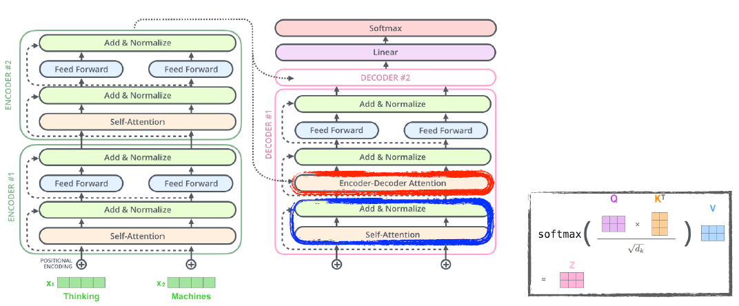
- In the decoder, the self-attention layer is only allowed to attend to earlier positions in the output sequence which is done by masking future positions before the softmax step.
- The “Encoder-Decoder Attention” layer works just like multi-headed selfattention, except it creates its Queries matrix from the layer below it, and takes the Keys and Values from the encoder stack.
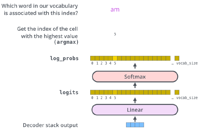
- The final layer converts the stack of decoder outputs to the distribution over words.
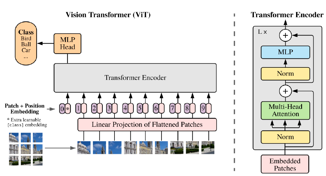
Vision Transformer
Vision 쪽에서도 Transformer가 활용되어 image detection에 쓰이기도 한다.
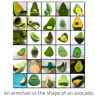
- 문장을 해석하여 이미지를 만들기도 한다.