RNN

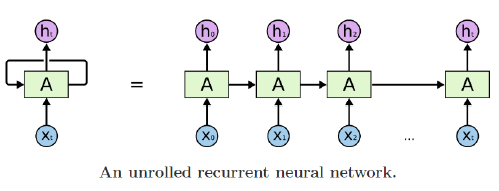
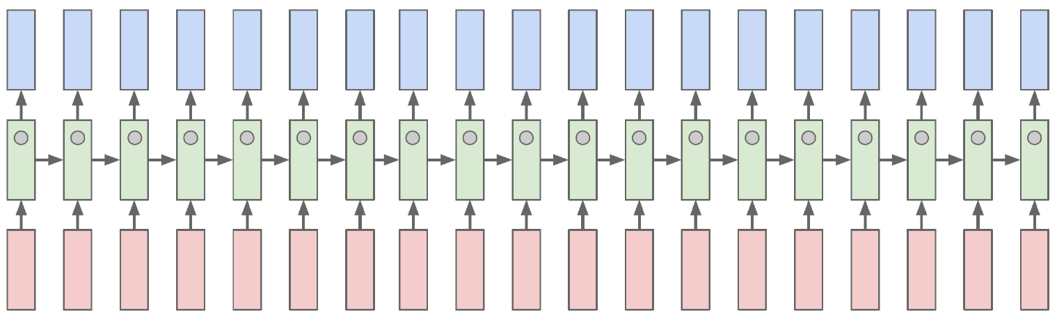
• Basic structure

• Inputs and outputs of RNNs (rolled version)
  We usually want to predict a vector at some time steps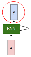

  

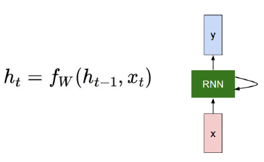
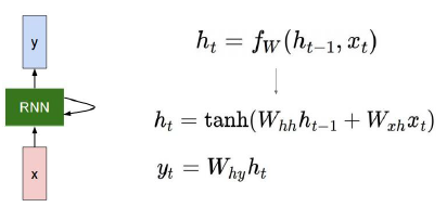
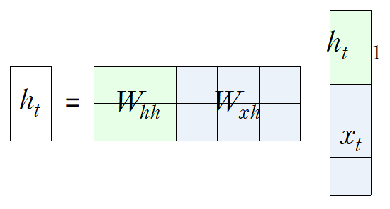
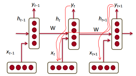
• How to calculate the hidden state of RNNs
  We can process a sequence of vectors by applying a recurrence formula at every time step
  
  $ℎ_{𝑡−1}$: old hidden-state vector
  $𝑥_𝑡$: input vector at some time step
  $ℎ_𝑡$: new hidden-state vector
  $𝑓_𝑊$: RNN function with parameters W
  $𝑦_𝑡$: output vector at time step t

• Notice
  The same function and the same set of parameters are used at every time step
  

• The state consists of a single “hidden” vector h

• $h_t$ 2차원 벡터, $h_{t-1}$ 2차원 벡터, $x_t$ 3차원 벡터

---

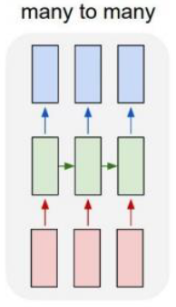
Types of RNNs

• One-to-one: Standard Neural Networks

• One-to-many: Image Captioning
  첫 입력이 주어지고 나면 각 hidden state의 input은 0으로 채워진 벡터를 준다.

• Many-to-one: Sentiment Classification

• Sequence-to-sequence: Machine Translation

• Sequence-to-sequence: Video classification on frame level

---

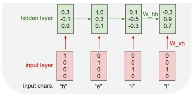
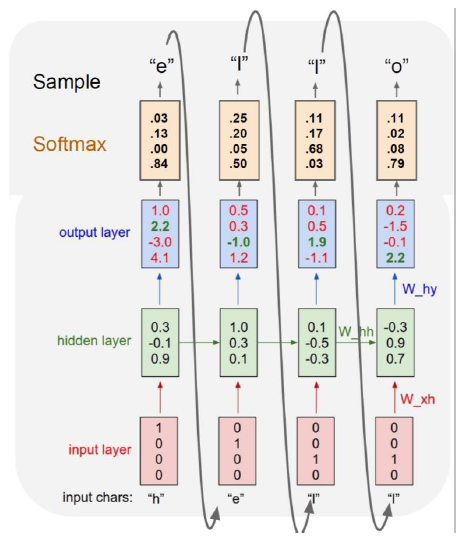
Character-level Language Model

Example of training sequence “hello”

• Vocabulary: [h, e, l, o]
• Example training sequence: “hello”

• $h_t = \operatorname{tanh}(W_{hh}h_{t-1} + W_{xh}x_t + b)$

• $\operatorname{Logit} = 𝑊_{ℎ𝑦}ℎ_𝑡 + 𝑏$

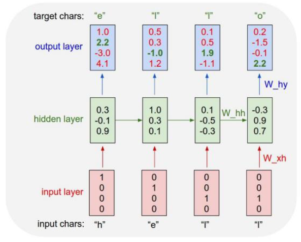
• At test-time, sample characters one at a time, feed back to model

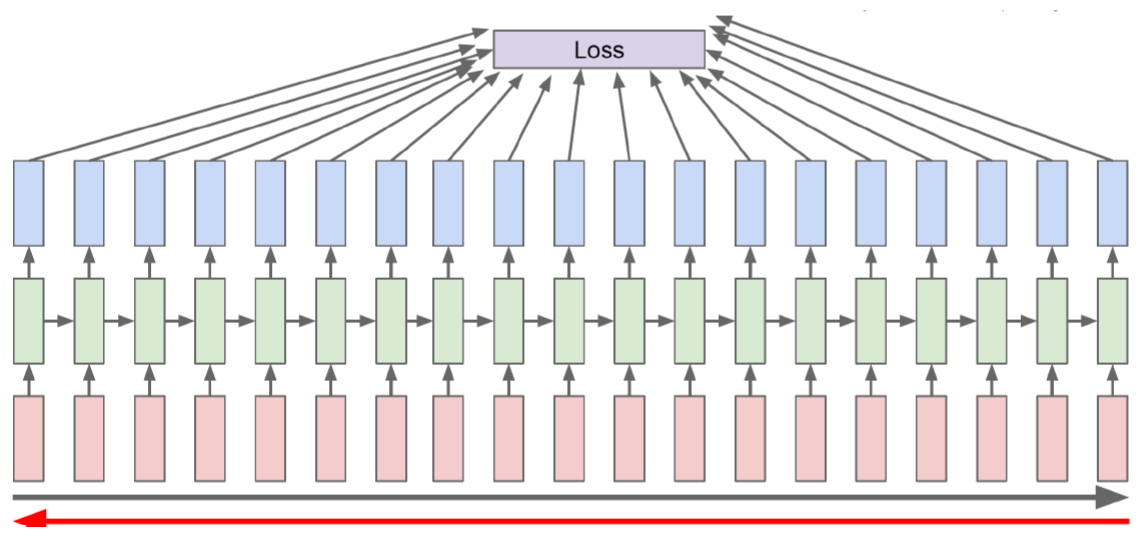
Backpropagation through time (BPTT)

• Forward through entire sequence to compute loss, then backward through entire sequence to comput gradient

• Run forward and backward through chunks of the sequence instead of whole sequence
  GPU의 연산량에는 한계가 있어 조금씩 잘라서 학습한다. 이때 forward network는 연결시키고 backward를 할 때는 자른다.

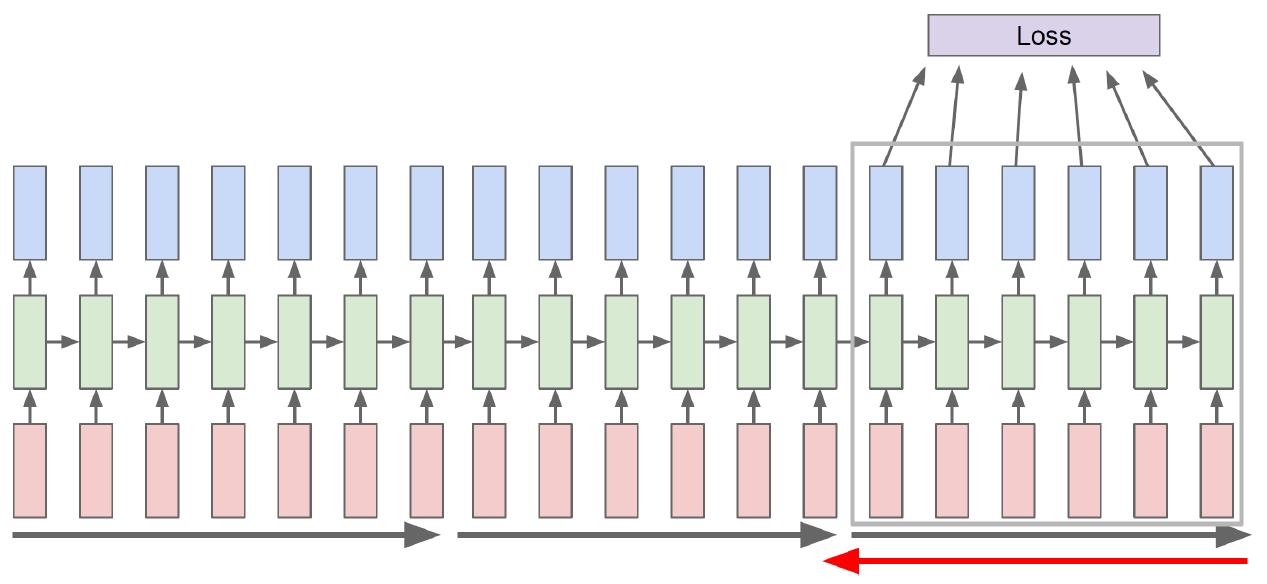
• Carry hidden states forward in time forever, but only backpropagate for some smaller number of steps

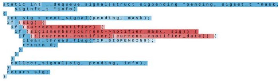
Searching for Interpretable Cells

Hidden state cell 벡터 중 하나의 차원을 고정하고 분석한다.

• How RNN works
  Hideen state cell의 특정 차원의 값이 음수면 파란색, 양수면 빨간색으로 표시된다.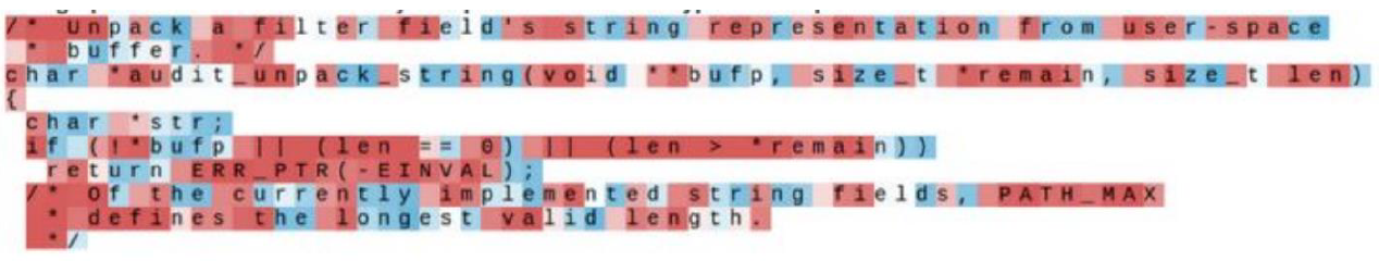

  

• Quote detection cell
  따옴표가 열리고 닫히는 것에 따라 특정 차원의 역할을 확인할 수 있다. (따옴표의 열리고 닫힘을 기억)

  

• If statement cell

  

---

Vanishing/Exploding Gradient Problem

RNN is excellent, butvMultiplying the same matrix at each time step during backpropagation causes gradient vanishing or exploding.

• Toy Example
  $ℎ_𝑡 = \operatorname{tanh}(𝑤_{𝑥ℎ}𝑥_𝑡 + 𝑤_{ℎℎ}ℎ_{𝑡−1} + 𝑏)$, $𝑡 = 1,2,3$

  For $𝑤_{ℎℎ} = 3$, $𝑤_{𝑥ℎ} = 2$, $𝑏 = 1$
  $ℎ_3 = \operatorname{tanh}(2𝑥_3 + 3ℎ_2 + 1)$
  $ℎ_2 = \operatorname{tanh}(2𝑥_2 + 3ℎ_1 + 1))$
  $ℎ_1 = \operatorname{tanh}(2𝑥_1 + 3ℎ_0 + 1))$
  ...
  $ℎ_3 = \operatorname{tanh}(2𝑥_3 + 3 \operatorname{tanh} (2𝑥_2 + 3ℎ_1 + 1) + 1)$
  

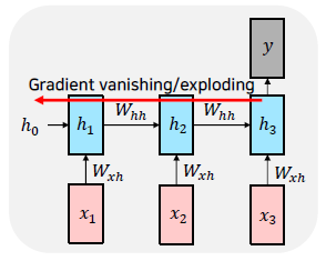
  $w_{hh}$가 1보다 크면 back propagation 에서 계속 곱해지므로(chain rule) gradient exploding이 일어나고, 1보다 작으면 gradient vanishing이 일어난다.

• https://imgur.com/gallery/vaNahKE
  위 링크를 누르면 $W_{hh}$ 행렬(정사각형 모양의 행렬)의 변화 패턴을 보여준다. (일반적으로 $W_{hh}$는 정방 행렬 - 길이는 Hidden_state의 길이)
  time step(정사각형 위의 숫자)을 거슬러 올라갈 수록(층이 줄어들 수록) 공비가 1보다 작을 경우 chain rule에 의해 gradient가 감소하는 것을 보여준다.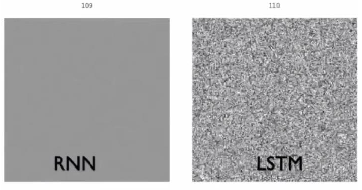

  

LSTM & GRU

LSTM

Long Short-Term Memory

• Core Idea: pass cell state information straightly without any transformation
  Solving long-term dependency problem

• What is LSTM (Long Short-Term Memory)?
  단기기억을 더 오래 가져간다.(Gradient vanishing 문제를 개선)

• RNN과 LSTM

  network	expression
  RNN	$h_t=f_w(x_t, h_{t-1})$
  LSTM	$\{C_t, h_t\} = \operatorname{LSTM}(x_t, C_{t-1}, h_{t-1})$

  $h$는 hidden state, $C$는 cell state를 나타낸다. LSTM에서 $h$는 $C$를 가공해서 만들어진다.

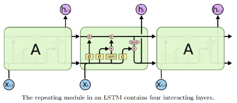
• Long short-term memory
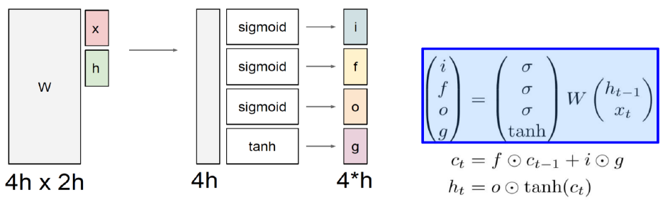
  i: Input gate, Whether to write to cell
  f: Forget gate, Whether to erase cell
  o: Output gate, How much to reveal cell
  g: Gate gate, How much to write to cell

• $h$와 $x$의 차원을 각 각 h라 하면 $w$의 column은 2h가 되고, 그 결과가 4개의 h로 sigmoid, sigmoid, sigmoid, tanh를 통과하기 때문에 row는 4h가 된다. sigmoid는 0 ~ 1 사이의 값이기 때문에, 과거의 정보를 어떤 비율로 가져갈지 결정한다. tanh는 -1 ~ 1 사이의 값이기 때문에 현재 time step에서 계산되는 유의미한 정보를 정한다.
  

• A gate exists for controlling how much information could flow from cell state
  i, f, o, g는 각각 다음 state로 가는 $C$와 $h$를 가공하는 역할을 한다.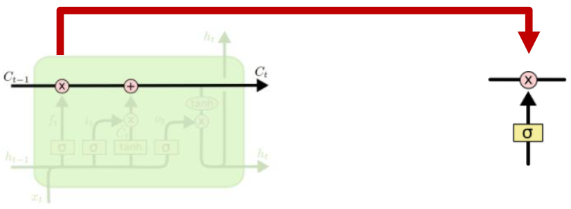

  

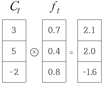
Forget gate

$𝑓_𝑡 = \sigma(𝑊_𝑓 \cdot [ℎ_{𝑡−1}, 𝑥_𝑡] + 𝑏_𝑓)$

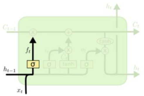
$h_{t-1}$과 $x_t$의 선형결합으로 만들어진 $f_t$ [0.7, 0.4, 0.8]가 $C_t$ [3, 5, -2]와 성분곱이 된다. 이 때 $f_t$의 각 성분을 과거의 정보를 70% 기억, 40% 기억, 80% 기억한다고 말할 수 있다.

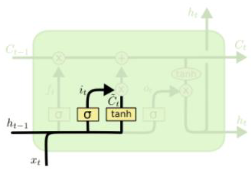
Input gate & Gate gate

Generate information to be added and cut it by input gate
$𝑖_𝑡 = \sigma (𝑊_𝑖 \cdot [ℎ_{𝑡−1}, 𝑥_𝑡] + 𝑏_𝑖)$
$\tilde{𝐶}_𝑡 = \operatorname{tanh}(𝑊_𝐶 \cdot [ℎ_{𝑡−1}, 𝑥_𝑡] + 𝑏_𝐶)$

Generate new cell state by adding current information to previous cell state
$𝐶_𝑡 = 𝑓_𝑡 \cdot 𝐶_{𝑡−1} + 𝑖_𝑡 \cdot \tilde{𝐶}_𝑡$

forget gate를 거친 $C_{t-1}$ 과 $\tilde{C}_t$를 바로 더하지 않고, $i_t$를 곱해주고 더한다. 이는 $\tilde{C}_t$가 한번의 선형결합만 거쳤기 때문에, 한번 더 정보를 가공($i_t$)해서 더해주겠다는 의미로 이해하면 된다.

Output gate

Generate hidden state by passing cell state to tanh and output gate
Pass this hidden state to next time step, and output or next layer if needed
$𝑜_𝑡 = \sigma (𝑊_𝑜 \cdot [ℎ_{𝑡−1}, 𝑥_𝑡] + 𝑏_𝑜)$
$ℎ_𝑡 = 𝑜_𝑡 \cdot \operatorname{tanh}(𝐶_𝑡)$

$C_t$가 가진 정보를 각 차원 별로 얼마나 가져갈지 결정한다.

• $C_t$는 기억해야할 모든 정보를 담고 있는 벡터

• $h_t$는 현재 time step에서 예측값을 내는 output layer의 입력값으로 사용되는 벡터
  ($C_t$가 가진 많은 정보 중에서 현재 time step에 필요한 정보만을 filterling 한 벡터)

---

GRU

Gated Recurrent Unit

LSTM 모델 구조를 경량화해서 적은 메모리량과 빠른 계산이 가능

LSTM에 있던 cell state 벡터와 hidden state 벡터를 일원화해서 $h_t$, $h_{t-1}$만 존재

$𝑧_𝑡 = \sigma (𝑊_𝑧 \cdot [ℎ_{𝑡−1}, 𝑥_𝑡])$
$𝑟_𝑡 = \sigma (𝑊_𝑟 \cdot [ℎ_{𝑡−1}, 𝑥_𝑡])$
$\tilde{ℎ}_𝑡 = \operatorname{tanh}(𝑊 \cdot [𝑟_𝑡 \cdot ℎ_{𝑡−1}, 𝑥_𝑡] )$
$ℎ_𝑡 = (1 − 𝑧_𝑡) \cdot ℎ_{𝑡−1} + 𝑧_𝑡 \cdot \tilde{ℎ}_𝑡$
c.f) $𝐶_𝑡 = 𝑓_𝑡 \cdot 𝐶_{𝑡−1} + 𝑖_𝑡 \cdot \tilde{𝐶}_𝑡$ in LSTM

$z_t$가 [0.6, 0.3, 0.8] 이면 $1 - z_t$ 는 [0.4, 0.7, 0.2] 이기 때문에 항상 각 성분의 합은 1이다. input gate $z_t$가 커질 수록 forget gate $1 - z_t$의 값은 작아진다.

---

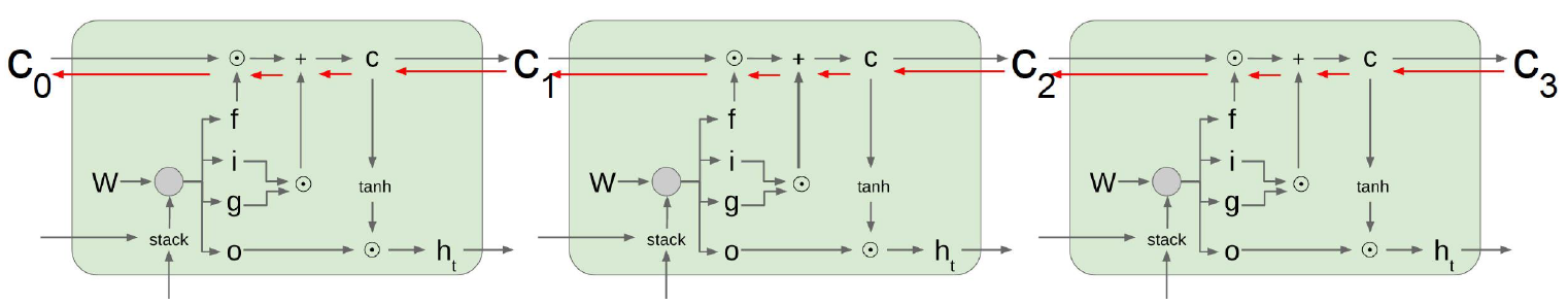
Backpropagation in LSTM & GRU

Uninterrupted gradient flow

$h_t$와 $C_t$가 계산되는 과정이 곱셈이 아닌 덧셈으로 진행되기 때문에 gradient explosion이나 gradient vanishing 현상이 없어졌다. (덧셈 연산은 back propagation 과정에서 gradient를 복사해준다)

---

Summary on RNN / LSTM / GRU

• RNNs allow a lot of flexibility in architecture design
• Vanilla RNNs are simple but don’t work very well
• Backward flow of gradients in RNN can explode or vanish
• Common to use LSTM or GRU: their additive interactions improve gradient flow