Seq2Seq with Attention

Seq2Seq Model

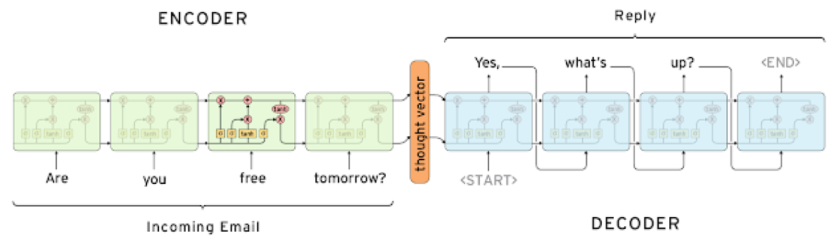
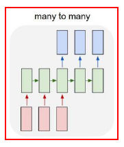
• It takes a sequence of words as input and gives a sequence of words as output

• It composed of an encoder and a decoder

• Machine Translation, Chat bot
  

• decoder의 첫 time step에 'SOS'(Start of String) 라는 토큰을 입력으로 주고 $h_0$는 Encoder에서 출력된 $h$를 사용한다. 출력값으로 'EOS'(End Of Sentence)가 출력되면 종료한다.

• LSTM의 각 hidden state 벡터의 차원은 고정되어있는데, sequence가 길어질수록 처음 정보는 점차 유실될 수 있다. 예를 들어, $h$가 3차원 벡터라면 3차원 공간에 과거의 모든 정보를 담아야 하기 때문에 정보가 점차 유실된 다는 것이다.
  'I go home.' 문장을 번역하려고 할 때, sequence가 길어지면 I의 정보가 유실되어 '나는' 이라는 출력이 안 나올 수 있다. 이런 문제를 해결하기 위해 'home go I'처럼 문장을 뒤집어서 입력으로 주는 시도도 있었다.

Seq2Seq Model with Attention

• Attention provides a solution to the bottleneck problem

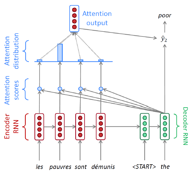
• Core idea: At each time step of the decoder, focus on a particular part of the source sequence.
  핵심 아이디어는 각각의 time step에서 출력된 결과는 가장 최근에 입력된 벡터를 가장 잘 반영하고 있다는 것이다. 그래서 각 hidden state의 결과를 종합해서 decoder에서 활용해보자는 아이디어이다.

• https://google.github.io/seq2seq/
  위 링크를 들어가면 Attention이 sequence에서 어떻게 적용되는지 확인할 수 있다.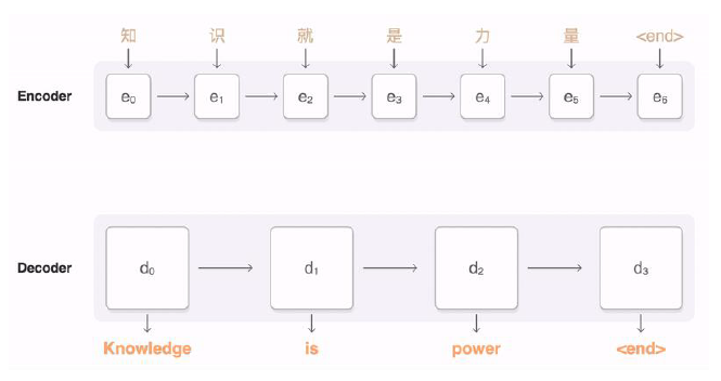

  

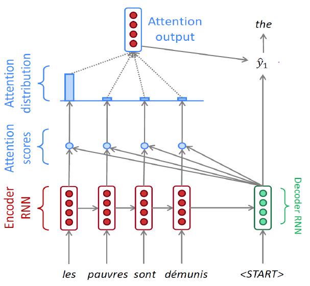
• Use the attention distribution to take a weighted sum of the encoder hidden states

• The attention output mostly contains information the hidden states that received high attention

• Decoder에서 나온 hidden state 벡터를 encoder의 각 hidden state와 내적을 하고, softmax를 통과시킨다. softmax를 통과해서 얻어지는 벡터는 attention vector라고 부르며 이 때 얻은 가중치 벡터를 이용해서 hidden state 벡터들의 가중평균을 하여 Attention output을 얻는다. decoder의 output과 가장 연관이 높은 encoder의 hidden state를 찾는 과정이라고 생각할 수 있다.

• Attention output은 context vector로도 부른다. (맥락에 대한 정보를 포함)

• Concatenate attention output with decoder hidden state, then use to compute $\hat{𝑦}_1$ as before
  Attention ouput 벡터와 decoder의 output vector를 concat 시켜output layer의 입력으로 사용한다.

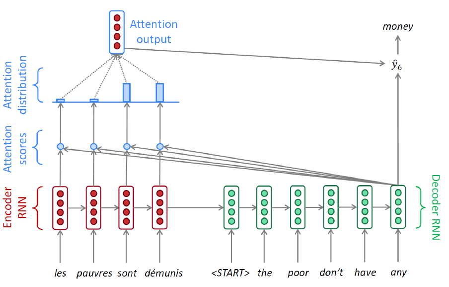
• 학습할 때 Decoder를 살펴보면 <start> 입력을 받은 RNN의 출력을 다시 다음 RNN의 입력값으로 넣어주는게 아니라 ground truth인 the를 넣어주는데 이를 teacher forcing이라고 한다. 항상 정답을 매 입력마다 넣어주기 때문에 실제 상황과는 다르기 때문에, teacher forcing을 통해 학습을 하다가 예측이 정확해지면, tearch forcing을 사용하지 않고 학습을 진행한다.

Different Attention Mechanisms

$\operatorname{score}(h_t, \bar{h}_s)= \begin{cases} {h_t}^T \bar{h}_s & \operatorname{dot}\\ {h_t}^T W_a \bar{h}_s & \operatorname{general}\\ {v_a}^T \operatorname{tanh}(W_a[h_t; \bar{h}_s]) & \operatorname{concat} \end{cases}$

• ${h_t}^T \bar{h}_s$
  기본적인 내적
  
  

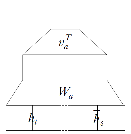
end to end learning

가공하는 과정도 학습시킨다.

• ${h_t}^T W_a \bar{h}_s$
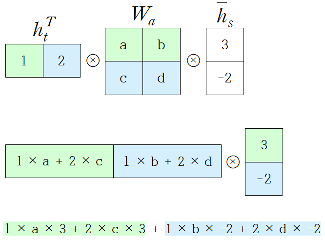
  같은 차원, 다른 차원 끼리의 곱과 그 가중치를 더한 내적
  

• ${v_a}^T \operatorname{tanh}(W_a[h_t; \bar{h}_s])$
  

Attention의 장점

• Attention significantly improves NMT performance

  • It is useful to allow the decoder to focus on particular parts of the source

• Attention solves the bottleneck problem
  encoder의 마지막 hidden state만 decoder의 input으로 제공하기 때문에 긴 sequence에서는 과거 데이터의 보존이 힘들어 진다.

  • Attention allows the decoder to look directly at source; bypass the bottleneck

• Attention helps with vanishing gradient problem

  • Provides a shortcut to far-away states
    
    만약 money가 아닌 다른 단어가 생성이 되면 그 결과가 back propagation을 통해전달 된다. 이 때 encoder의 hidden state vector의 초반 time step까지 전달하는 경우 attention이 없다면 decoder의 마지막 time step부터 하나하나 거슬러 뒤로 가야하지만, Attention output을 통해 빠르게 hiddens state로 gradient를 전달해줄 수 있다.

• Attention provides some interpretability

  • By inspecting attention distribution, we can see what the decoder was focusing on
    decoder가 encoder의 어느 부분을 더 잘 반영하는지 확인할 수 있다.
  • The network just learned alignment by itself

Attention Examples in Machine Translation

• It properly learns grammatical orders of words
• It skips unnecessary words such as an article

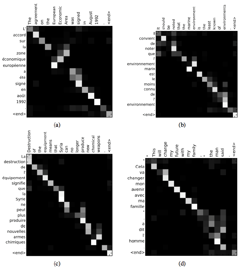
위 그림을 보면 행이 encoder 입력, 열이 decoder의 출력을 나타내는데 각 출력이 encoder의 어느 부분을 참고했는지 확인할 수 있다.

Beam search

• Greedy decoding has no way to undo decisions!
  Seq2Seq with Attention에서는 다음 단어만을 예측하는 task를 학습하고 매 time step마다 단어 중 가장 확률이 높은 것만을 선택해서 decoding을 진행한다. sequence로서의 전체적인 문장의 확률값을 보는게 아니라 근시안적으로 현재 time step에서 가장 좋아보이는 단어를 그 때 그 때 선택한다.

  • Input: il a m’entarté (he hit me with a pie)
    $\rightarrow$ he ___
    $\rightarrow$ he hit ___
    $\rightarrow$ he hit a ___ (whoops, no going back now…)

• How can we fix this?
  
  

• Ideally, we want to find a (length 𝑇) translation 𝑦 that maximizes

  • $𝑃(𝑦 |𝑥) = 𝑃 (𝑦_1 |𝑥) 𝑃 (𝑦_2 |𝑦_1, 𝑥) 𝑃 (𝑦_3| 𝑦_2, 𝑦_1, 𝑥) \dots 𝑃 (𝑦_𝑇 |𝑦_1, \dots , 𝑦_{𝑇−1}, 𝑥 ) = \prod_{1}^{T} 𝑃(𝑦_𝑡 |𝑦_1,\dots , 𝑦_{𝑡−1}, 𝑥)$
    x를 입력 문장, y를 출력문장이라고 할 때, 첫 step의 출력이 $y_1$으로 나오더라도, 뒤의 조건부 확률의 곱이 작게되면 전체적인 확률 값은 낮을 수 있다.
    

• We could try computing all possible sequences $𝑦$
  모든 가능한 경우를 확인할 수는 있지만, Vocab size만큼의 연산을 반복 시행하게 되어, 연산량이 기하급수적으로($V^t$) 커지게 된다.

  • This means that on each step $𝑡$ of the decoder, we are tracking $𝑉^𝑡$ possible partial translations, where $𝑉$ is the vocabulary size
  • This O($𝑉^𝑡$) complexity is far too expensive!

---

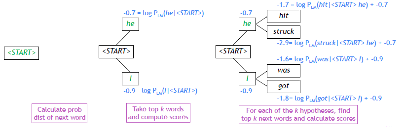
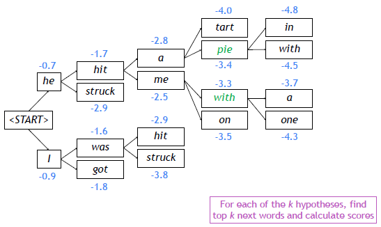
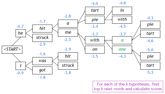
Beam Search

Core idea

On each time step of the decoder, we keep track of the 𝑘 most probable partial translations (which we call hypothese)

• $k$ is the beam size (in practice around 5 to 10)

• A hypothesis $𝑦_1, \dots , 𝑦_𝑡$ has a score of its log probability

  $\operatorname{score}(𝑦_1, \dots , 𝑦_𝑡) = \operatorname{log}P_{LM}(y_1, \dots, y_t|x) = \sum_{i=1}^{t}\operatorname{log} 𝑃_{𝐿𝑀}( 𝑦_i|y_1, \dots , 𝑦_{i-1}, 𝑥)$
  • Scores are all negative, and a higher score is better
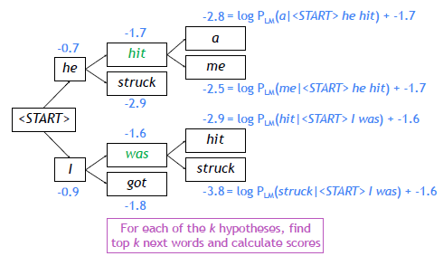
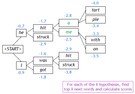
  • We search for high-scoring hypotheses, tracking the top k ones on each step

• Beam search is not guaranteed to find a globally optimal solution. But it is much more efficient than exhaustive search!

Stopping criterion

• In greedy decoding, usually we decode until the model produces a <END> token
  • For example: <START> he hit me with a pie <END>
    
    
• In beam search decoding, different hypotheses may produce <END> tokens on different timesteps
  • When a hypothesis produces <END>, that hypothesis is complete
  • Place it aside and continue exploring other hypotheses via beam search
    
    
• Usually we continue beam search until:
  • We reach timestep $T$ (where $T$ is some pre-defined cutoff), or
  • We have at least $n$ completed hypotheses (where $n$ is the pre-defined cutoff)

Finishing up

• We have our list of completed hypotheses

• How to select the top one with the highest score?

• Each hypothesis $𝑦_1, \dots , 𝑦_𝑡$ on our list has a score

  $\operatorname{score}(𝑦_1, \dots , 𝑦_𝑡) = \operatorname{log}P_{LM}(y_1, \dots, y_t|x) = \sum_{i=1}^{t}\operatorname{log} 𝑃_{𝐿𝑀}( 𝑦_i|y_1, \dots , 𝑦_{i-1}, 𝑥)$

• Problem with this: longer hypotheses have lower scores
  확률은 0 ~ 1 사이의 값이기 때문에 곱해서 log를 취하면, 길이가 긴 sequence일 수록 더 낮은 값을 갖게된다.

• Fix: Normalize by length

  $\operatorname{score}(𝑦_1, \dots , 𝑦_𝑡) = \cfrac{1}{t}\sum_{i=1}^{t}\operatorname{log} 𝑃_{𝐿𝑀}( 𝑦_i|y_1, \dots , 𝑦_{i-1}, 𝑥)$

BLEU score

Precision and Recall

Reference: Half of my heart is in Havana ooh na na
Predicted: Half as my heart is in Obama ooh na

정밀도
검색엔진에서 검색어를 입력했을 때 검색된 문서 중에 그 내용이 들어간 문서가 얼마나 검색되었는지

재현율
검색엔진에서 검색어를 입력했을 때 실제 그 내용이 들어간 문서 중에 얼마나 검색되었는지

조화평균 더 낮은 값에 가중치를 둬서 평균을 구한다

• Predicted (from model 1)
  Half as my heart is in Obama ooh na

• Reference
  Half of my heart is in Havana ooh na na

• Predicted (from model 2)
  Havana na in heart my is Half ooh of na

  Metric	Model 1	Model 2
  Precision	78%	100%
  Recall	70%	100%
  F-measure	73.78%	100%

  Flaw: no penalty for reordering

  
  

BLEU score

BiLingual Evaluation Understudy (BLEU)

• N-gram overlap between machine translation output and reference sentence

• Compute precision for n-grams of size one to four

• Add brevity penalty (for too short translations)

  $\operatorname{BLEU = min(1, \cfrac{length\_of\_prediction}{length\_of\_reference})(\prod_{i = 1}^{4} precision_i)^{\frac{1}{4}}}$
  • Typically computed over the entire corpus, not on single sentences
    
    

• 기하평균: $\operatorname{\prod_{i = 1}^{4} (precision_i)^{\frac{1}{4}}}$
  I love this movie very much
  나는 이 영화를 (정말) 많이 사랑한다.
  어느정도 문맥이 맞으면 더 정확하다고 판단하는 precision을 사용한다.
  그리고 낮은 값에 가중치를 주기 위해 기하평균을 사용한다. (조화평균은 지나치게 낮은 값에 가중치를 부여한다)
  
  

• graivity penalty: $\operatorname{min(1, \cfrac{length\_of\_prediction}{length\_of\_reference})}$
  단순히 길이만을 고려했을 때, ground truth 보다 짧으면 짧아진만큼 precision을 더 낮춰준다.

• Example
  Predicted (from model 1): Half as my heart is in Obama ooh na
  Reference: Half of my heart is in Havana ooh na na
  Predicted (from model 2): Havana na in heart my is Half ooh of na

  Metric	Model 1	Model 2
  Precision (1-gram)	$\cfrac{7}{9}$	$\cfrac{10}{10}$
  Precision (2-gram)	$\cfrac{4}{2}$	$\cfrac{0}{9}$
  Precision (3-gram)	$\cfrac{2}{7}$	$\cfrac{0}{8}$
  Precision (4-gram)	$\cfrac{1}{6}$	$\cfrac{0}{7}$
  Brevity penalty	$\cfrac{9}{10}$	$\cfrac{10}{10}$
  BLEU	$0.9 \times \sqrt{3} / 3 = 52 \%$	0