Transformer

Transformer: High-Level View

• Attention is all you need, NeurIPS’17
  No more RNN or CNN modules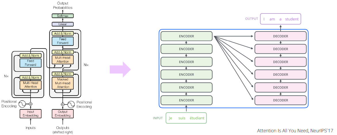

  
  

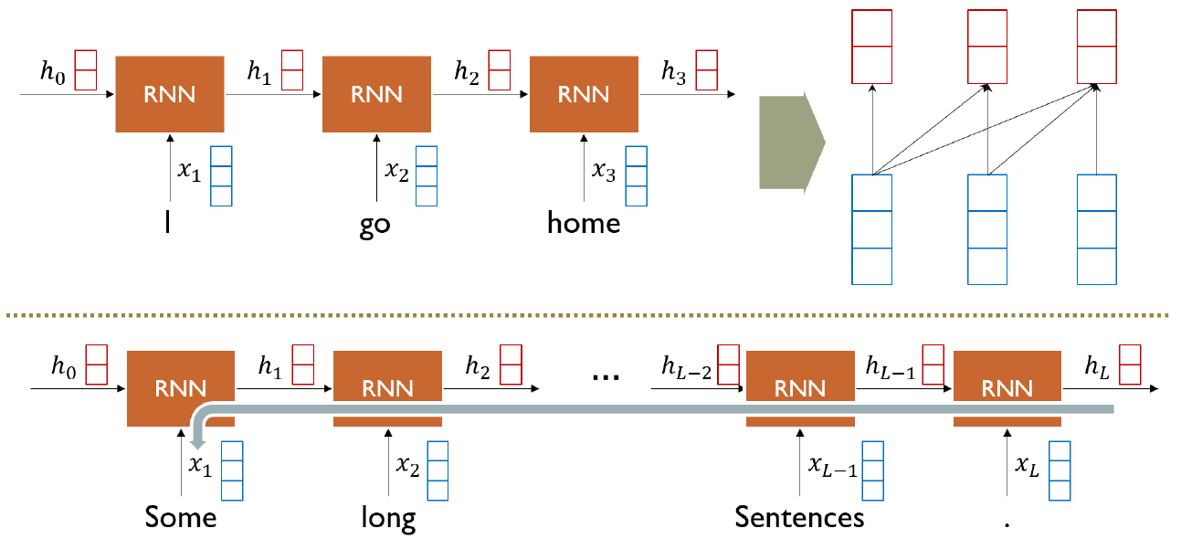
RNN: Long-Term Dependency

상대적으로 먼 과거의 정보는 잘 반영하지 못 한다.
(gradient vanishing, gradient explosion)

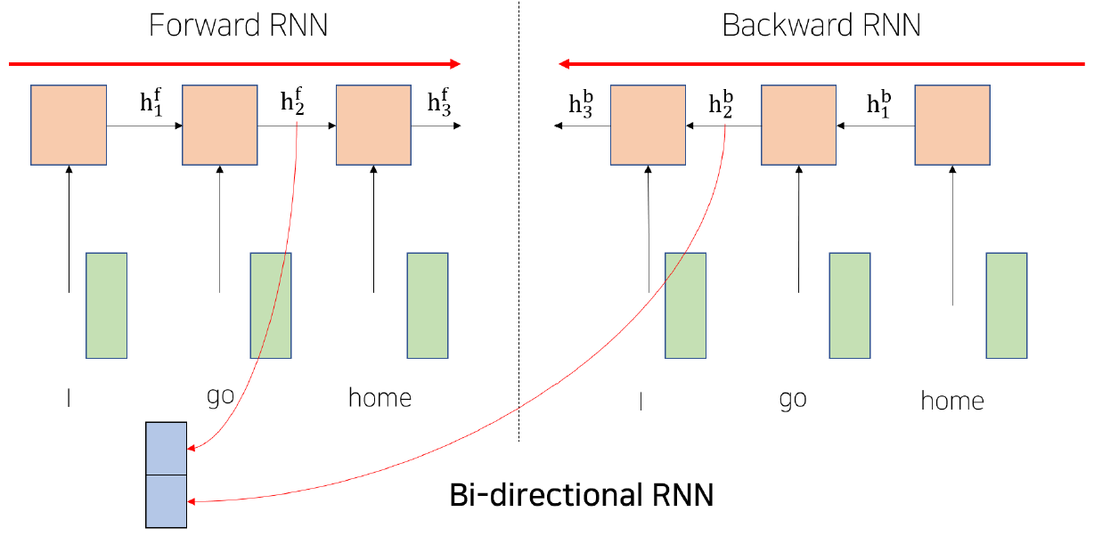
Bi-Directional RNNs

Sequence가 time step의 형태로 진행되기 때문에 앞단의 hidden state는 자기 자신의 정보만 알 뿐, 아직 뒤에 있는 hidden state들의 정보는 반영하지 않는다. 이를 해결하기 위해 양방으로 RNN을 구성하여 각 hidden state의 정보를 반영하도록 고안한 방법

Transformer: Long-Term Dependency

Seq2Seq with Attention에서 decoder에서 나오는 $h_d$를 encoder에서 나오는 $h_e$와 내적해서 나오는 Attention output을 encoder와 decoder 구분 없이 그냥 encoder 단에서 수행해도 되지 않을까하는 아이디어

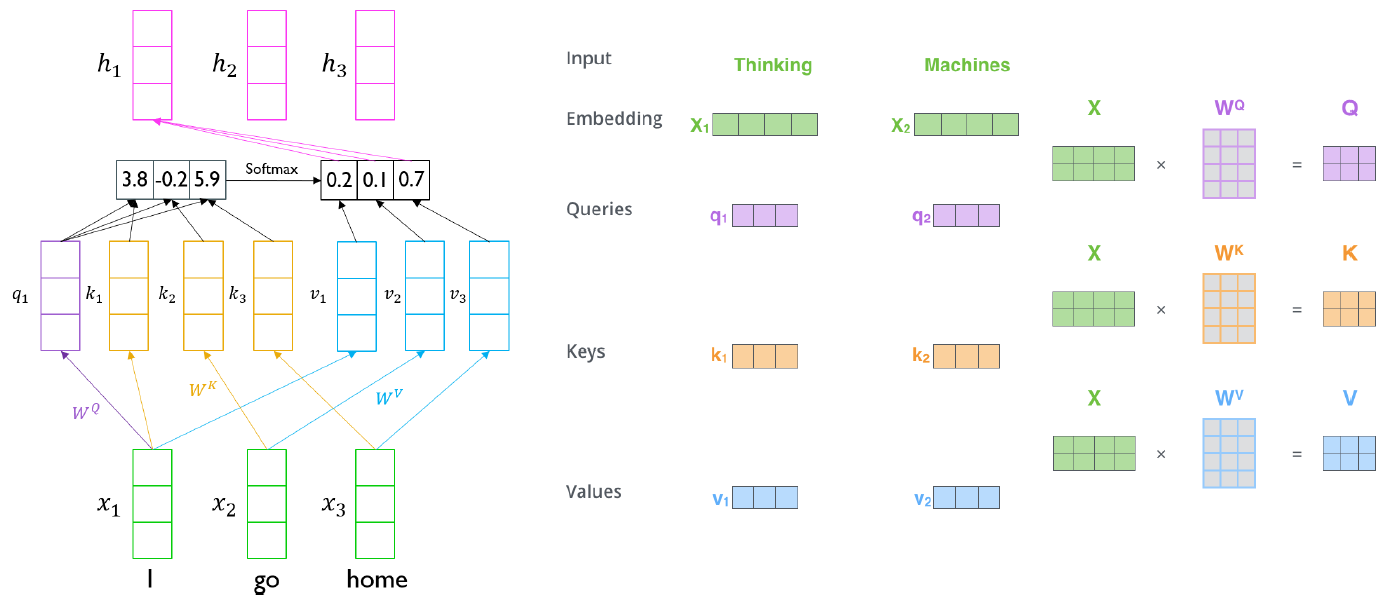
• 각 벡터가 decoder의 $h_d$처럼 사용되고 모든 벡터들이 $h_e$처럼 사용되어 자기 자신과 내적, 다른 벡터와 내적을 통해 Attention 벡터를 얻게된다. decoder와 encoder 구분 없이 자기 자신의 벡터만을 이용해서 Attention을 생성하기에 이를 Self - Attention module 이라고 부른다. 그러나 보통 자기 자신과 내적을 했을 때 나오는 유사도가 서로 다른 벡터들과 내적을 했을 때 나오는 유사도보다 훨씬 크게 나온다. 결국 자기 자신에게 큰 가중치가 걸리기 때문에 Attention 벡터가 나타나게 되고 이를 이용하여 encoding을 진행하여 나온 벡터들도 결국 자기 자신의 정보만을 주로 갖고 있게 된다.

• Query 벡터
  decoder의 hidden state와 같은 역할을 하는 벡터

• Key 벡터
  encoder의 각 hidden state와 같은 역할을 하는 벡터

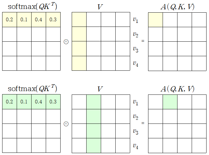
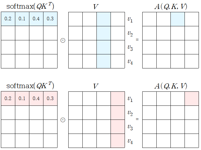
• Value 벡터
  key와 query의 내적을 softmax를 통과시켜 얻은 값을 가중평균할 때 사용되는 벡터

---

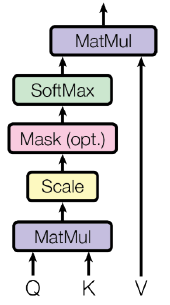
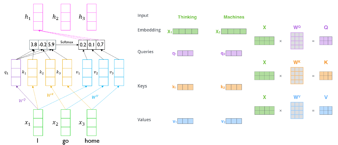
Transformer: Scaled Dot-Product Attention

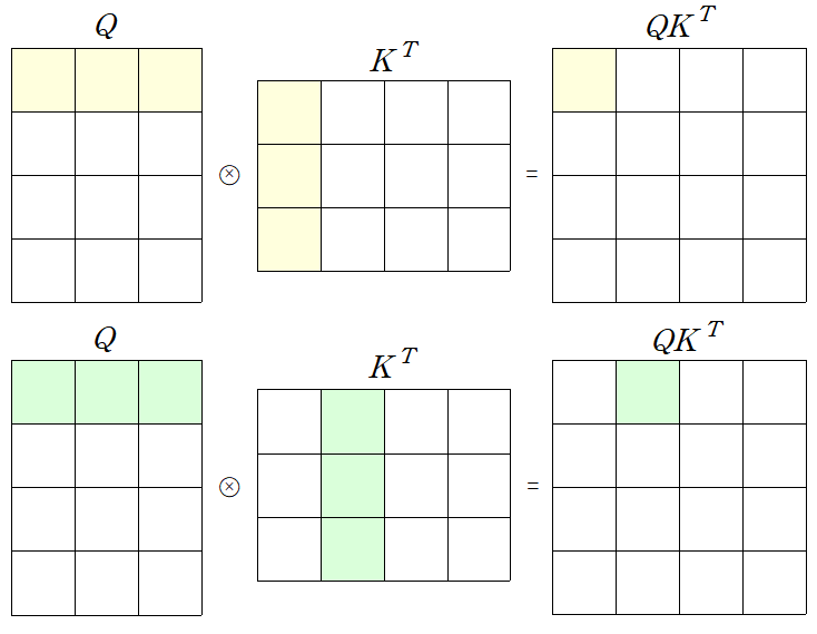
• Inputs: a query $𝑞$ and a set of key-value $(𝑘, 𝑣)$ pairs to an output
• Query, key, value, and output is all vectors
• Output is weighted sum of values
• Weight of each value is computed by an inner product of query and corresponding key
• Queries and keys have same dimensionality $𝑑_𝑘$, and dimensionality of value is $𝑑_𝑣$

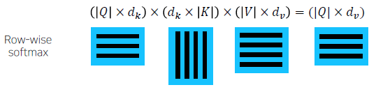
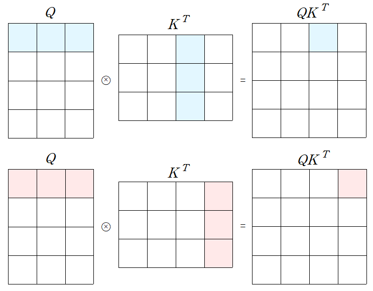
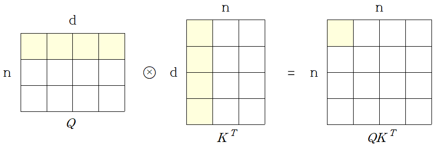
• When we have multiple queries 𝑞, we can stack them in a matrix 𝑄

  $A(q, K, V) = \sum_{i} \cfrac{exp(q \cdot k_i)}{\sum_j exp(q \cdot k_j)} v_i$

• Becomes

  $A(Q, K, V) = \operatorname{softmax}(QK^T)V$

  행렬로 바꾸어 연산을 수행하면 gpu를 이용하여 연산(병렬적인 연산)을 수행할 수 있어 연산 속도가 더 빠르다.

  

  

  

  

  

  

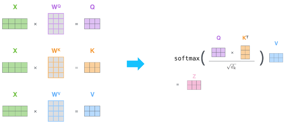
• 실제 Transformer 구현 상으론 동일한 shape로 mapping된 Q, K, V가 사용되어 각 matrix의 shape는 모두 동일하다.

• Example from illustrated transformer
  

• Problem

  • As $𝑑_𝑘$ gets large, the variance of $𝑞^𝑇𝑘$ increases
  • Some values inside the softmax get large
  • The softmax gets very peaked
  • Hence, its gradient gets smaller

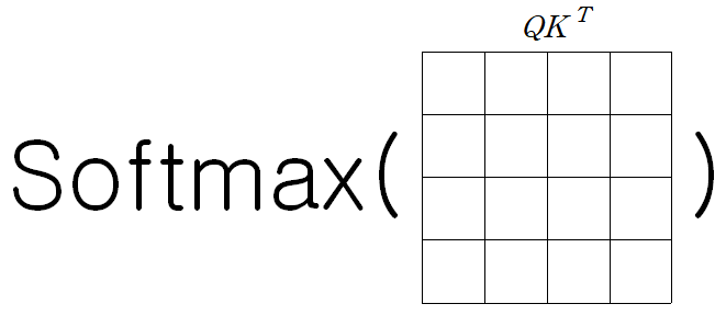
  $d_k$의 차원이 증가할수록 분산이 커지게 되어 softmax를 통과한 값의 확률 분포가 굉장히 큰 값에 몰리게 된다. 그렇게되면 gradient vanishing이 일어날 수 있다.
  예를 들어 평균이 0, 분산이 1인 독립인 $Q = [a, b]$와 $K = [x, y]$가 있으면 각 성분을 곱한 $qk$는 평균은 0 이지만 분산은 2 가 된다.

• Solution

  • Scaled by the length of query / key vectors:
    $A(Q, K, V) = \operatorname{softmax}(\cfrac{𝑄𝐾^𝑇} {\sqrt {𝑑_𝑘}})V$
    따라서 차원이 증가 할수록 분산이 커지게 되어 softmax($QK^T$)의 성분 중 하나가 큰 가중치를 갖게되어, 학습이 잘 안 되게 된다.
    그래서 softmax 확률분포의 표준편차를 1로 만들기위해 $\sqrt{d_k}$로 나눈다.(scaling) 그 결과 확률분포가 고르게 편성되어 학습이 안정화된다.

Transformer (Seq2Seq)

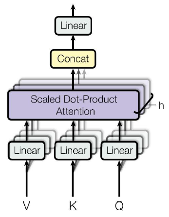
Transformer: Multi-Head Attention

• The input word vectors are the queries, keys and values

• In other words, the word vectors themselves select each other

• Problem of single attention

  • Only one way for words to interact with one another

• Solution

  • Multi-head attention maps $Q, K, V$ into the $h$ number of lower-dimensional spaces via $W$ matrices

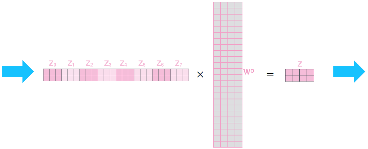
• Then apply attention, then concatenate outputs and pipe through linear layer

  $\operatorname{MultiHead} (𝑄, 𝐾, 𝑉) = \operatorname{Concat} (head_1, \dots , head_ℎ) 𝑊^O$
  $\operatorname{where} \;head_𝑖 = \operatorname{Attention}(𝑄𝑊_𝑖^𝑄, 𝐾𝑊_𝑖^𝐾, 𝑉𝑊_𝑖^𝑉 )$

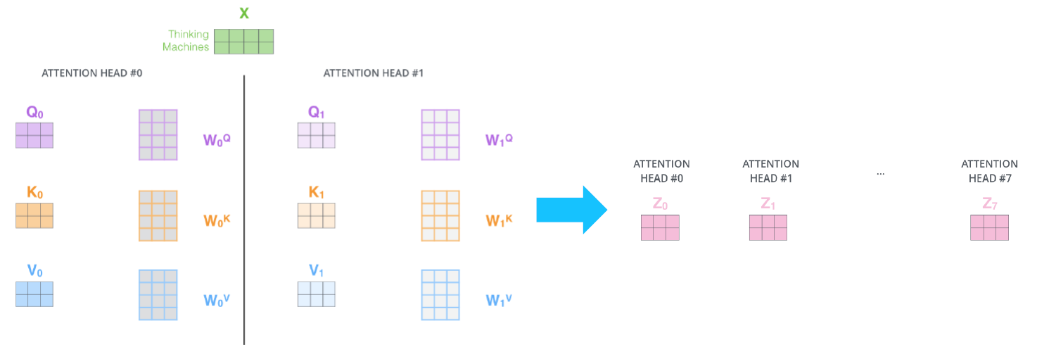
  Multi-Head Attention은 Attention module(head)을 여러개 둔다. 즉 여러개의 서로 다른 $\operatorname{A(Q, K, V)}$ 가 생성되고 모두 concat된다.

  

• Example from illustrated transformer
  

  
  

• Maximum path lengths, per-layer complexity and minimum number of sequential operations for different layer types

  • $n$ is the sequence length
  • $d$ is the dimension of representation
  • $k$ is the kernel size of convolutions
  • $r$ is the size of the neighborhood in restricted self-attention
    
    

    Layer Type	Complexity per Layer	Sequential Operations	Maximum Path Length
    Self-Attention	$O(n^2 \cdot d)$	$O(1)$	$O(1)$
    Recurrent	$O(n \cdot d^2)$	$O(n)$	$O(n)$
    Convolutional	$O(k \cdot n \cdot d^2)$	$O(1)$	$O(\operatorname{log}_k(n))$
    Self-Attention (restricted)	$O(r \cdot n \cdot d)$	$O(1)$	$O(n/r)$

  
  

Self-Attention

곱셈연산이 d번, 총 $n \times n$의 행렬성분마다 계산되기 때문에 연산량(메모리 사용량)은 $O(n \cdot d^2)$이 된다.

RNN

$d$의 값은 hidden state dimension으로 사용자가 임의로 정할 수 있지만, $n$은 sequence의 갯수로 사용자가 정할 수 없다. 그래서 입력데이터 sequence의 길이가 길수록 Self-Attention의 메모리 사용량은 $n^2$에 비례하기 때문에 메모리 사용량이 많아진다. 그러나 메모리가 충분하다면 Self-Attention은 병렬처리가 가능하여 빠른 속도로 연산이 가능하다. RNN의 경우에는 각 time step이 처리가 되어야 다음 time step의 연산이 가능하기 때문에 병렬화가 불가능하다.

Maximum path length는 RNN의 경우 첫번째 sequence가 마지막 sequence에 영향을 주려면 time step의 갯수 n 만큼 거쳐야 한다. Self-Attention은 key와 value에서 정보를 얻기 때문에 한번에 접근할 수 있다. 그래서 Self-Attention은 Long Term Dependency의 문제를 근본적으로 해결할 수 있다.

---

Transformer: Block-Based Model

• Each block has two sub-layers
  • Multi-head attention
  • Two-layer feed-forward NN (with ReLU)
    
    
• Each of these two steps also has
  • Residual connection and layer normalization:
  • $LayerNorm(x + sublayer(x))$

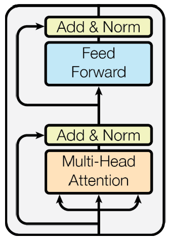
위 그림에서 Multi-Head Attention으로 들어가는 세 개의 화살표는 Value, Key, Query에 해당한다.

Add는 ResNet에 있던 Residual connection을 이용한 것이다. 예를 들어, Attention output이 $\begin{pmatrix} 2 & 3 & -1 \\ 3 & 5 & 1 \end{pmatrix}$ 이고, Input이 $\begin{pmatrix} 1 & 5 & 2 \\ -4 & 1 & 3 \end{pmatrix}$ 이라면, Add 된 값은 $\begin{pmatrix} 3 & 8 & 1 \\ -1 & 6 & 4 \end{pmatrix}$ 가 된다. 이 때 주의할 점은 input 벡터와 Attention output 벡터의 dimension이 동일해야한다는 점이다. (그래야 각 dimension 별로 연산이 가능하다.)
바꾸어 말하면, Attention은 Add된 출력값이 $\begin{pmatrix} 3 & 8 & 1 \\ -1 & 6 & 4 \end{pmatrix}$가 나오도록 하려고 Attention module의 내부 파라미터들이 학습된다는 뜻이다. 즉, $\begin{pmatrix} 2 & 3 & -1 \\ 3 & 5 & 1 \end{pmatrix}$ 을 출력하도록 학습된다. 또한, 이러한 과정을 통해 gradient vanishing 문제도 해결된다.

---

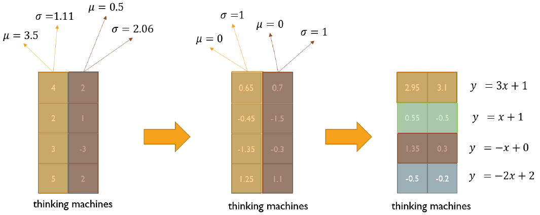
Transformer: Layer Normalization

Layer normalization changes input to have zero mean and unit variance, per layer and per training point (and adds two more parameters)

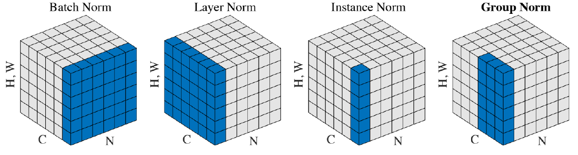
Batch Norm

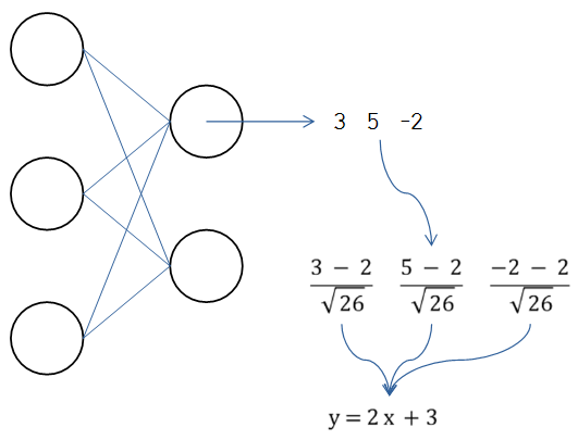
batch size가 3, dimension이 3이 input으로 주어질 때 hidden layer 첫번째 노드의 output을 3, 5, -2 라고 하면, 이를 평균을 0, 표준편차는 1로 바꿔준다. 그리고 Affine transformation 이라는 $y = 2x + 3$ 연산을 수행한다. 그러면 평균이 3만큼, 분산은 4가 된다. 이 때 2와 3을 파라미터로 정하면 최적화된 평균, 분산을 얼마로 할지 학습하게 된다.

Layer Norm

Layer normalization consists of two steps:

• Normalization of each word vectors to have mean of zero and variance of one.
• Affine transformation of each sequence vector with learnable parameters

---

Transformer: Positional Encoding

위의 Transformer model은 입력 sequence에 상관없이 항상 같은 attention vector를 출력한다. 즉, go home I를 입력값으로 줘도 go, home, I에 해당하는 output 벡터들이 각 I go home으로 했을 때의 I, go, home에 해당하는 벡터와 같아진다. (가중치평균을 구하는 과정은 교환법칙이 성립한다) 그래서 여기에 위치에 대한 정보를 입력하기 위해 Positional Encoding을 해준다.

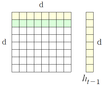
• Use sinusoidal functions of different frequencies
  $𝑃𝐸_{(pos,2i)} = sin(pos/10000^{2i/d_{model}} )$
  $𝑃𝐸_{(pos,2i+1)} = cos(pos/10000^{2i/d_{model}} )$
• Easily learn to attend by relative position, since for any fixed offset $k$, $PE_{(pos+k)}$ can be represented as linear function of $PE_{(pos)}$

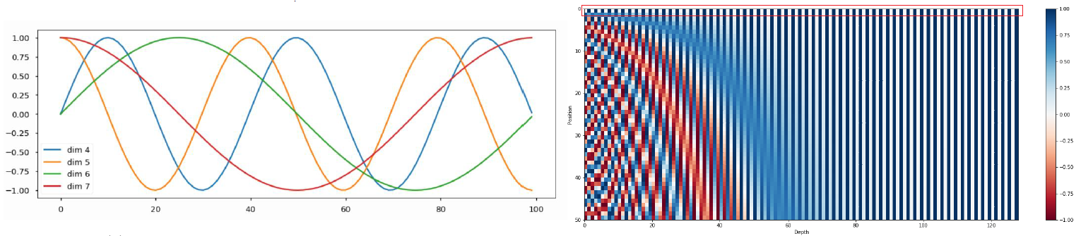
오른쪽 그림에서 각 position 별 벡터(row 벡터)가 원래의 output 벡터에 더해져 Positional Encoding 된다.

---

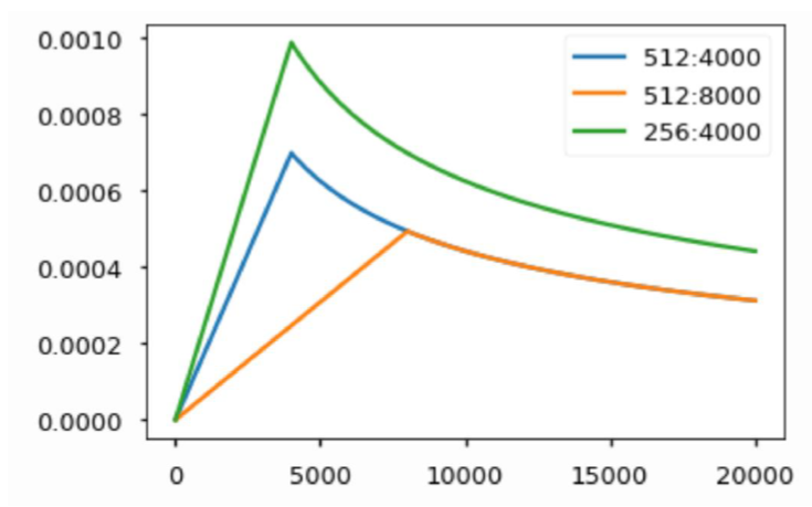
Transformer: Warm-up Learning Rate Scheduler

Adam 같은 Optimizer들은 lr(learning rate)값을 고정해주는데 이를 iteration에 따라 동적으로 바꿔준다.
$learning rate = d_{model}^{-0.5} \cdot min(\#𝑠𝑡𝑒𝑝^{−0.5}, \;\#𝑠𝑡𝑒𝑝 \cdot warmup\_steps^{−1.5})$

Transformer: High-Level View

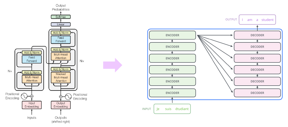
Input → Input Embedding → Positional Encoding → Multi-Head Attention → Add & Norm → Feed Forward → Add & Norm 로 구성되는 Layer를 총 N층으로 쌓는다. (N은 주로 6, 12, 24로 쓰인다)

---

Transformer: Encoder Self-Attention Visualization

Words start to pay attention to other words in sensible ways

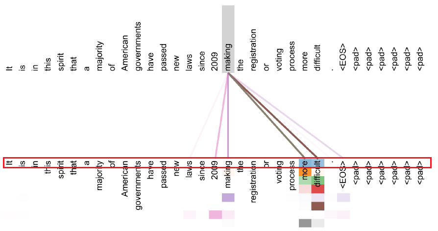
위 그림은 making을 Query로 사용할 때 Attention이 어떻게 반영되는지 보여준다. 이 때 빨간색으로 테두리되어 있는 부분은 $Head_1$의 Attention이 반영된 부분을 나타낸다. 즉, 각 Head의 Attention을 다르게 반영한다는 듯이다. 처음 5개 정도의 Head에는 more과 difficult에 Attention이 많이 되고 있다. 또한 자기자신(marketing)을 Attention하는 Head가 존재하기도 하고, 시기 정보(2009)를 Attention하는 Head가 존재하는 것도 확인된다.

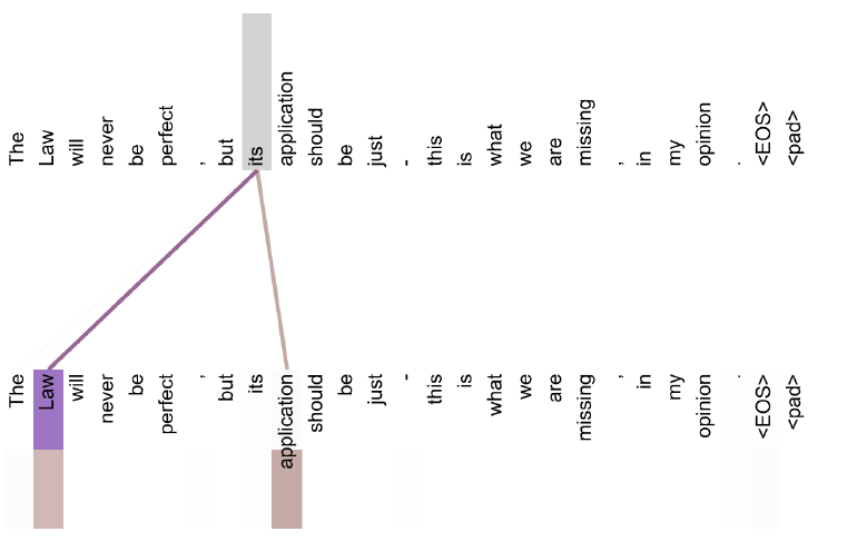
위 그림에서 its가 Query로 사용되면, its가 Law를 가리키고 있다고 보여주는 Attention Head와 its를 한정해주는 application에 Attention Head가 동작하는 것이 확인 된다.

https://colab.research.google.com/github/tensorflow/tensor2tensor/blob/master/tensor2tensor/notebooks/hello_t2t.ipynb

위 링크에 들어가면 앞선 그림들과 같은 Attention 패턴을 볼 수 있다.

---

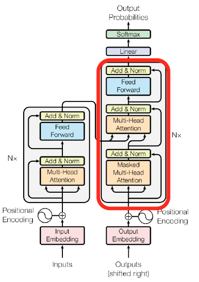
Transformer: Decoder

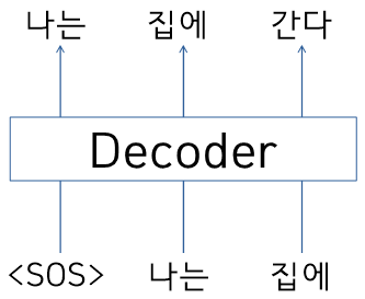
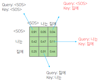
학습 당시에 '<SOS>' '나는' '집에' sequence가 decoder의 입력 embedding 벡터로 주어진다. 이때 <SOS>의 output으로 '나는', '나는'의 output으로 '집에', '집에'의 output으로 '간다'가 나와야한다.

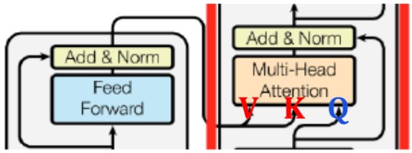
'<SOS>' '나는' '집에' 세 벡터는 Masked Mutli-Head Attention을 지나 다음 Multi-Head Attention의 Query로, Encoder에서 나온 각 벡터들이 Value와 Key로 주어진다.

이후 FCL(Full Connected Layer)의 Linear transformation 층을 지나 softmax를 통과하여 vocab에 해당하는 벡터로 출력된다. 이 때 vocab의 크기가 10만개라면 10만 차원의 벡터가 생성된다.

• Two sub-layer changes in decoder
• Masked decoder self-attention on previously generated outputs

• Encoder-Decoder attention, where queries come from previous decoder layer and keys and values come from output of encoder

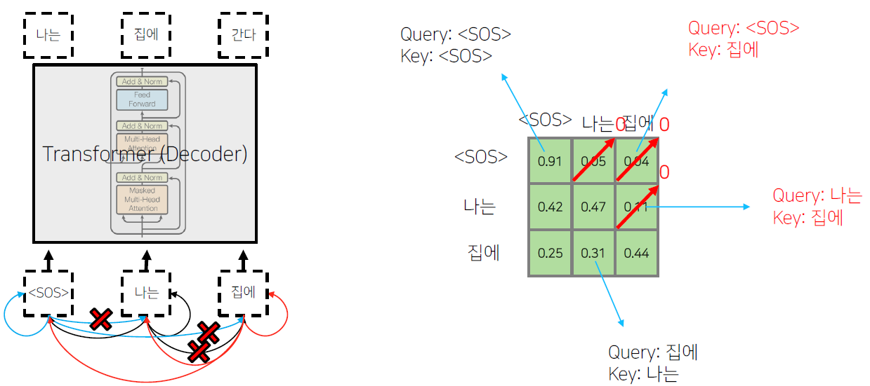
Transformer: Masked Self-Attention

• Those words not yet generated cannot be accessed during the inference time
• Renormalization of softmax output prevents the model from accessing ungenerated words

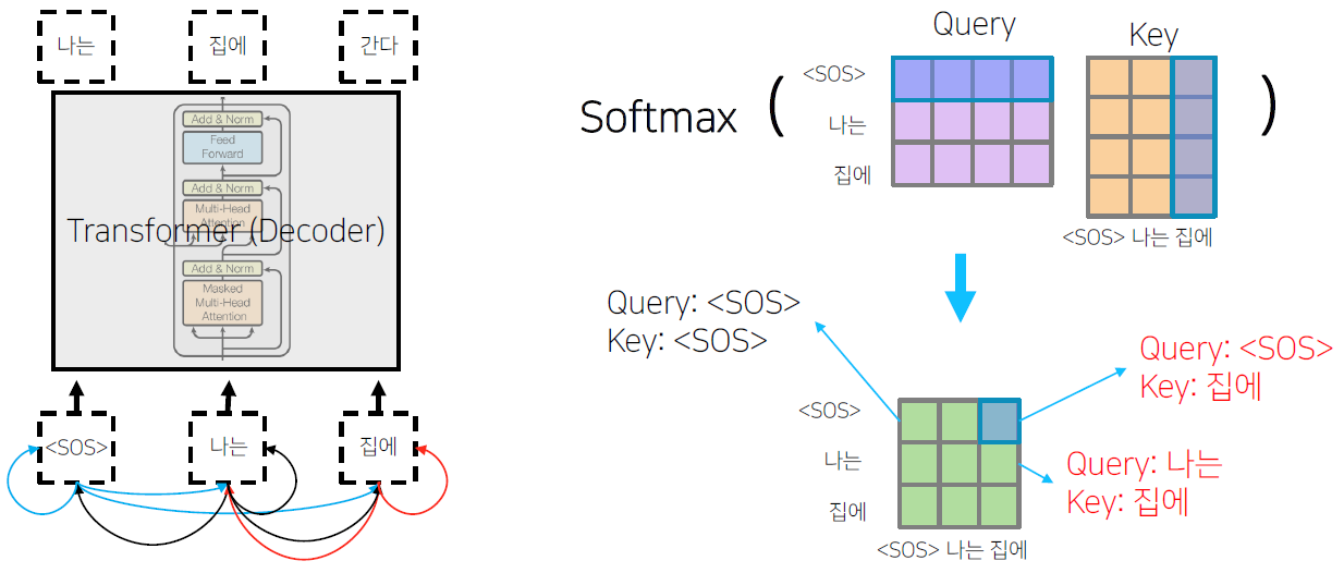
'<SOS>'가 '<SOS>', '나는', '집에' 에 대해서 self-attention encoding을 하는 중에 정보의 가능여부를 확인해야 한다. 학습 과정에서는 모든 입력이 주어지지만, 예측 과정에서는 첫번째 time step에서 '<SOS>' 까지만 주어져있을 때 '나는'을 예측해야 하고, 두번째 time step 에서 '<SOS>' 와 '나는' 까지 주어졌을 때 '집에'를 예측해야 한다. 즉, 첫번째 time step 에서 '<SOS>'가 '나는' 과 '집에' 에 접근하는 것은 불가능하다. 그렇기 때문에 '<SOS>' 를 Query로 사용할 때 접근가능한 Key와 Value에서 '나는' 과 '집에' 를 제외해야 한다.

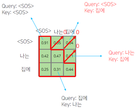
이 때 0이 되지 않는 값들을 row 별로 합이 1이 되도록 normalization 해준다. 합으로 각 성분들을 나줘준다.

즉 Masking의 의미는 Attention을 할 때는 모두가 모두를 볼 수 있도록 한 후, 보면 안 되는(뒤에서 나오는) 단어에 대한 Attention의 가중치를 후처리적으로 0으로 만들어준다. 이후 value 벡터와 가중평균을 구한다.

---

Transformer: Experimental Results

Results on English-German/French translation (newstest2014)

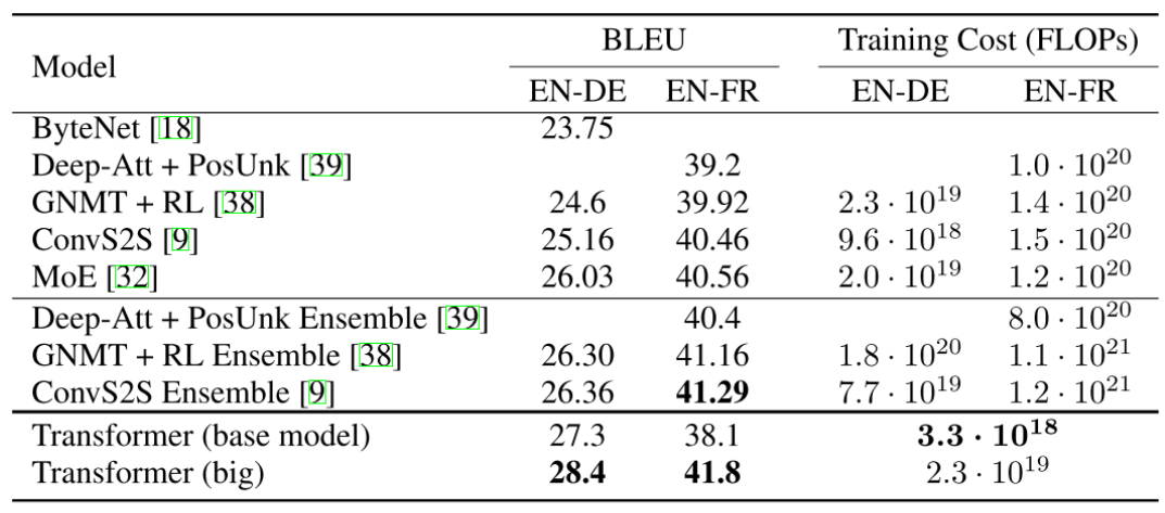
Transformer의 성능을 보면 BLEU score가 20 ~ 40 정도의 성능을 갖는 것을 알 수 있다. 그러나 이는 보기와는 다르게 높은 성능을 갖는다. 예를 들어, '나는 수학을 열심히 공부한다.' 라는 문장이 있을 때(Ground truth), '나는 열심히 수학을 공부한다.' 라는 번역 문장이 예측값으로 주어지는 경우에는 두 문장이 결국 동일한 의미의 문장이지만, bi-gram, tri-gram, four-gram을 따졌을 때는 precision 값이 낮아지게 된다.