지난 포스팅에서 Genetic Algorithm을 활용해서 하이퍼파라미터 최적화(weights), 이미지 재생성 실습을 진행했습니다.
하지만, Genetic Algorithm은 Artificial Neural Networks를 훈련하기 위해 사용될 수도 있습니다. PyGAD는 pygad.gann.GANN와 pygad.gacnn.GACNN 모듈을 통해 neural networks, convolutional neural networks 훈련을 지원합니다.
pygad.gann모듈은 Genetic Algorithm을 사용해서 분류문제(Classification) 혹은 회귀문제(Regression)를 해결하기 위해 neural networks를 훈련합니다. 훈련을 위해, pygad와 pygad.nn 두 모듈을 사용합니다.
이번 포스팅에서는 분류 문제에 대한 신경망 훈련을 위해 이 pygad.gann.GANN 모듈을 사용해볼 것입니다. 이 예제에서는 XOR 논리 게이트를 시뮬레이션하는 네트워크를 구축합니다.
XOR 연산이란?
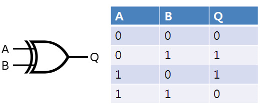
XOR 연산이란, 두 개의 연산자 중 하나만이 1일때, 1을 반환합니다. 위의 그래프는 XOR 연산을 그래프로 표현한 것입니다.
XOR 연산을 신경망으로 표현하면, A,B input 데이터를 받는 input layer, 그리고 여러개의 hidden layers, 마지막 분류(0 or 1) 결과를 나타내는 output layer로 정의할 수 있습니다.
우선 라이브러리들을 다운받아줍니다.
!pip install pygad==2.17.0
import numpy
import pygad
import pygad.nn
import pygad.gann
Training Dataset 준비
신경망을 구축하고 훈련시키기 전에 훈련 데이터(입력 및 출력)를 준비해야 합니다. 훈련 데이터의 입력과 출력은 NumPy 배열입니다.
만약 200개의 sample 데이터가 있고, 각 sample 데이터에 50개의 feature가 있는 경우, input 데이터의 구성은 (200, 50)입니다. 현재 예시에서는 4개의 sample 데이터와, 각 sample 데이터에 2개의 feature(A,B)가 있으므로 (4, 2) 구성을 가집니다.
output 배열에 대해서 각 요소는 샘플의 클래스 레이블을 나타내는 하나의 숫자형 데이터로 표현되어야 합니다.
data_inputs = numpy.array([[1, 1],
                           [1, 0],
                           [0, 1],
                           [0, 0]])

data_outputs = numpy.array([0,
                            1,
                            1,
                            0])
input의 수는 2개, 분류를 위한 레이블은 0 또는 1이므로 2개로 정의합니다.
num_inputs = data_inputs.shape[1]
num_classes = 2
pygad.gann.GANN class의 인스턴스 생성
훈련 데이터를 준비하고 나서, pygad.gann.GANN 클래스의 인스턴스를 생성합니다. num_solutions는 genetic algorithm population에 20개의 솔루션이 있음을 의미합니다. 즉 GA의 개념에 빗대어 표현하면, 모집단의 크기(population size)와 같습니다. 이 20개의 신경망은 동일한 아키텍처를 갖습니다.
num_neurons_input: Input Layer는 2개의 뉴런을 가짐(2개의 features)num_neurons_hidden_layers: 각 Hidden Layer는 2개의 뉴런을 가짐num_neurons_output: Output Layer는 2개의 뉴런을 가짐(클래스 레이블, 0 or 1)
num_solutions = 20

GANN_instance = pygad.gann.GANN(num_solutions=num_solutions,
                                num_neurons_input=num_inputs,
                                num_neurons_hidden_layers=[2],
                                num_neurons_output=num_classes,
                                hidden_activations=["relu"],
                                output_activation="softmax")
input layer와 hidden layer 사이에는 (number inputs x number of hidden neurons) = (2x2)와 같은 크기의 weights matrix가 있습니다.
hidden layer와 output layer 사이에는 (number of hidden neurons x number of outputs) = (2x2)와 같은 크기의 weights matrix가 있습니다.
Population Weights를 벡터화
XOR 문제에 대한 networks training 작업을 위해 population의 각 네트워크의 weights는 벡터로 표시되지 않고 각각 크기가 2x2인 2개의 행렬로 표시됩니다.
population weights를 각 네트워크마다 하나씩 벡터로 보유하는 목록을 생성하려면 pygad.gann.population_as_Vectors() 함수가 사용됩니다.
population_vectors = pygad.gann.population_as_vectors(population_networks=GANN_instance.population_networks)
initial_population = population_vectors.copy()
Fitness Function 정의
Fitness Function은 예측 정확도를 최대화하려고 시도합니다. 높은 Fitness value가 더 좋은 solution을 의미합니다.
pygad.nn.predict() 함수는 현재 solution의 weights를 사용해서 class의 레이블을 예측합니다. 또한, 예측을 위해 네트워크의 각 layer의 training_weights 속성에서 사용할 수 있는 훈련된 weights를 사용합니다.
def fitness_func(solution, sol_idx):
    global data_inputs, data_outputs

    predictions = pygad.nn.predict(last_layer=GANN_instance.population_networks[sol_idx],
                                   data_inputs=data_inputs)
    correct_predictions = numpy.where(predictions == data_outputs)[0].size
    solution_fitness = (correct_predictions/data_outputs.size)*100

    return solution_fitness
Generation Callback Function 정의
각 세대가 지날수록, Fitness Function은 각 solution별 Fitness Value를 계산하기 위해 호출될 것입니다. 앞서 설명된 것과 같이, pygad.nn.predict() 함수는 현재 solution(population)의 훈련된 trained_weights를 사용해서 output을 예측하기 위해 사용됩니다. 따라서 이러한 속성은 각 세대 진화 이후, GA에 의해 진화된 weights 의해 업데이트되어야 합니다.
pygad.gann.population_as_matrices(): 현재 모집단을 vector 형식에서 matrix 형식으로 변환하여 작동합니다.update_population_trained_weights(): 모집단의 matrics를 받아 모집단 내 모든 solution에 대한 모든 레이어의trained_weights를 업데이트합니다.
last_fitness = 0
def callback_generation(ga_instance):
    global GANN_instance, last_fitness

    population_matrices = pygad.gann.population_as_matrices(population_networks=GANN_instance.population_networks,
                                                            population_vectors=ga_instance.population)
    GANN_instance.update_population_trained_weights(population_trained_weights=population_matrices)
    print("Generation = {generation}".format(generation=ga_instance.generations_completed))
    print("Fitness    = {fitness}".format(fitness=ga_instance.best_solution()[1]))
    print("Change     = {change}".format(change=ga_instance.best_solution()[1] - last_fitness))
    last_fitness = ga_instance.best_solution()[1].copy()
pygad.GA class를 활용하여 인스턴스 생성
# the GA parameters are defined here
num_parents_mating = 4
num_generations = 50
mutation_percent_genes = 5
parent_selection_type = "sss"
crossover_type = "single_point"
mutation_type = "random"
keep_parents = 1
init_range_low = -2
init_range_high = 5
ga_instance = pygad.GA(num_generations=num_generations,
num_parents_mating=num_parents_mating,
initial_population=initial_population,
fitness_func=fitness_func,
mutation_percent_genes=mutation_percent_genes,
init_range_low=init_range_low,
init_range_high=init_range_high,
parent_selection_type=parent_selection_type,
crossover_type=crossover_type,
mutation_type=mutation_type,
keep_parents=keep_parents,
callback_generation=callback_generation)GA 실행
ga_instance.run()output:
Generation = 1
Fitness    = 100.0
Change     = 100.0
Generation = 2
Fitness    = 100.0
Change     = 0.0
Generation = 3
Fitness    = 100.0
Change     = 0.0
...
Generation = 50
Fitness    = 100.0
Change     = 0.0
Plot results 확인
ga_instance.plot_result()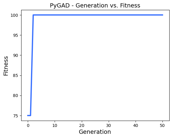
Best Solution 정보
# the GA searching results are illustrated
solution, solution_fitness, solution_idx = ga_instance.best_solution()
print("Parameters of the best solution : {solution}".format(solution=solution))
print("Fitness value of the best solution = {solution_fitness}".format(solution_fitness=solution_fitness))
print("Index of the best solution : {solution_idx}".format(solution_idx=solution_idx))
output:
Parameters of the best solution : [-3.17759453  0.0165431   1.66828862 -1.01964287 -4.03930743  0.33941187
  3.14860768 -0.16112557]
Fitness value of the best solution = 100.0
Index of the best solution : 0
# Tackle the generation of which the best fitness is appeared.
if ga_instance.best_solution_generation != -1:
print("Best fitness value reached after {best_solution_generation} generations.".format(best_solution_generation=ga_instance.best_solution_generation))output:
Best fitness value reached after 2 generations.Trained Weights를 사용해서 분류 예측
predictions = pygad.nn.predict(last_layer=GANN_instance.population_networks[solution_idx],
                               data_inputs=data_inputs)
print("Predictions of the trained network : {predictions}".format(predictions=predictions))
output:
Predictions of the trained network : [0, 1, 1, 0]통계 계산
num_wrong = numpy.where(predictions != data_outputs)[0]
num_correct = data_outputs.size - num_wrong.size
accuracy = 100 * (num_correct/data_outputs.size)
print("Number of correct classifications : {num_correct}.".format(num_correct=num_correct))
print("Number of wrong classifications : {num_wrong}.".format(num_wrong=num_wrong.size))
print("Classification accuracy : {accuracy}.".format(accuracy=accuracy))
output:
Number of correct classifications : 4.
Number of wrong classifications : 0.
Classification accuracy : 100.0.
이렇게 간단한 실습을 통해 GA를 사용해서 input(A,B)를 받아 XOR 논리연산 결과를 클래스 레이블로 분류하는 neural network를 만들어보았습니다.
다음 포스팅에서는, 이것을 더 연장해 2개의 input 데이터가 아니라 여러개의 input 데이터를 가지고 XOR 논리 연산 결과를 클래스 레이블로 분류하는 NN를 훈련해보는 시간을 갖도록 하겠습니다.