Sorting & Search

Binary Search

Binary Search

def binary_search(arr, target):
    low = 0
    high = len(arr) - 1

    while low <= high:
        mid = (low + high) // 2
        guess = arr[mid]

        if guess == target:
            return mid
        if guess > target:
            high = mid - 1
        else:
            low = mid + 1
    return None

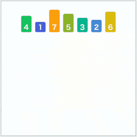
arr = [1, 3, 5, 7, 9]
target = 5

result = binary_search(arr, target)
if result is not None:
    print(f"Element found at index {result}")
else:
    print("Element not found in the array")

Bubble Sort

Bubble Sort

def bubble_sort(array):
    n = len(array)
    for i in range(n):
        for j in range(n - i - 1):
            if array[j] > array[j+1]:
                array[j], array[j+1] = array[j+1], array[j]
    return array

Time Complexity: O(N^2)

[4, 6, 2, 9, 1]  # 정렬되지 않은 배열

1단계 : [4, 6, 2, 9, 1] 
        4와 6을 비교

2단계 : [4, 6, 2, 9, 1]
           6과 2를 비교

3단계 : [4, 2, 6, 9, 1]
              6과 9를 비교

4단계 : [4, 2, 6, 9, 1]
                 9와 1를 비교

After making one rotation, the largest number, 9, came to the very end in this process.
Since we swapped the positions whenever a larger number appeared, it means it went to the very end. 
So, excluding the last digit, we just need to rotate again.

5단계 : [4, 2, 6, 1, 9]
        4와 2을 비교


6단계 : [2, 4, 6, 1, 9]
           4와 6을 비교

7단계 : [2, 4, 6, 1, 9]
              6와 1을 비교

Then, now the second largest number, 6, came to the second from the end. 
You only need to compare up to this point. There's no need to compare 6 and 9.

8단계 : [2, 4, 1, 6, 9]
        2와 4을 비교

9단계 : [2, 4, 1, 6, 9]
           4와 1을 비교

Now the third largest number, 4, came to the third from the end.

10단계 : [2, 1, 4, 6, 9]
         2와 1을 비교
         2 > 1 이므로 둘을 변경
        [1, 2, 4, 6, 9] 

Selection Sort

Selection Sort

def selection_sort(array):
    n = len(array)
    for i in range(n - 1):
        min_index = i
        for j in range(i+1, n):
            if array[j] < array[min_index]:
                min_index = j
        array[i], array[min_index] = array[min_index], array[i]

    return array

Time Complexity: O(N^2)

[4, 6, 2, 9, 1]  # 정렬되지 않은 배열

1단계 : [4, 6, 2, 9, 1] 
        4와 6과 2와 9와 1을 차례차례 비교
	      그 중 가장 작은 1과 맨 앞 자리인 4를 교체
       [1, 6, 2, 9, 4] 

자, 그러면 이제 가장 작은 숫자인 1이 맨 앞으로 왔습니다.
가장 작은 걸 가장 맨 앞으로 옮기기로 했으니까요!
그러면, 맨 앞자리를 제외하고 다시 한 번 반복하면 됩니다.

2단계 : [1, 6, 2, 9, 4]
           6과 2와 9와 4를 차례차례 비교
           그 중 가장 작은 2와 두번째 앞 자리인 6을 교체

3단계 : [1, 2, 6, 9, 4]
              6과 9와 4를 차례차례 비교
              그 중 가장 작은 4와 세번째 앞 자리인 6을 교체

4단계 : [1, 2, 4, 9, 6]
                 9와 6을 비교
                 그 중 가장 작은 6과 네번째 앞 자리인 9을 교체

Insertion Sort

Insertion Sort

def insertion_sort(array):

    for i in range(1, len(array)):
        key = array[i]
        j = i-1
        while j >=0 and key < array[j]:
            array[j + 1] = array[j]
            j -= 1
        array[j + 1] = key
    return array

Time Complexity: O(N^2)

[4, 6, 2, 9, 1]  # 정렬되지 않은 배열

1단계 : [4, 6, 2, 9, 1] 
        4는 현재 정렬되어 있는 부대원입니다. 
			  그럼 이제 새로운 신병인 6을 받습니다.
        4, 6 이 되는데 4 < 6 이므로 그대로 냅둡니다.
       [4, 6, 2, 9, 1] 이렇게요!

We've completed one rotation.
In this process, the new recruits, 4 and 6, are now in sorted order!
In this way, insertion sort becomes sorted after each rotation.

2단계 : [4, 6, 2, 9, 1]
        4, 6 은 현재 정렬되어 있는 부대원입니다.
        그럼 이제 새로운 신병인 2를 받습니다.
        4, 6, 2 가 되는데 6 > 2 이므로 둘을 변경합니다!
        4, 2, 6 가 되는데 4 > 2 이므로 둘을 변경합니다!
       [2, 4, 6, 9, 1] 이렇게요!

3단계 : [2, 4, 6, 9, 1]
        2, 4, 6 은 현재 정렬되어 있는 부대원입니다.
        그럼 이제 새로운 신병인 9를 받습니다.
        2, 4, 6, 9 가 되는데 6 < 9 이므로 그대로 냅둡니다.
       [2, 4, 6, 9, 1] 이렇게요!

4단계 : [2, 4, 6, 9, 1]
        2, 4, 6, 9 은 현재 정렬되어 있는 부대원입니다.
        그럼 이제 새로운 신병인 1을 받습니다.
        2, 4, 6, 9, 1 가 되는데 9 > 1 이므로 둘을 변경합니다!
        2, 4, 6, 1, 9 가 되는데 6 > 1 이므로 둘을 변경합니다!
        2, 4, 1, 6, 9 가 되는데 4 > 1 이므로 둘을 변경합니다!
        2, 1, 4, 6, 9 가 되는데 2 > 1 이므로 둘을 변경합니다!
       [1, 2, 4, 6, 9] 이렇게요!

However, there is a difference compared to bubble sort and selection sort.
While bubble sort and selection sort always take O(N^2) time, whether in the best or worst case scenarios,

In the best-case scenario, it takes Ω(N) time complexity.
This is because if an almost sorted array is inputted, it can escape without comparing with more elements due to the break statement.

Merge Sort

Merge Sort

Time complexity: O(Nlog_2N) = O(NlogN)

[5, 3, 2, 1, 6, 8, 7,  4] 이라는 배열이 있다고 하겠습니다. 이 배열을 반으로 쪼개면
[5, 3, 2, 1] [6, 8, 7, 4] 이 됩니다. 또 반으로 쪼개면
[5, 3] [2, 1] [6, 8]  [7, 4] 이 됩니다. 또 반으로 쪼개면
[5] [3] [2] [1] [6] [8] [7] [4] 이 됩니다.

이 배열들을 두개씩 병합을 하면 어떻게 될까요?
[5] [3] 을 병합하면 [3, 5] 로
[2] [1] 을 병합하면 [1, 2] 로
[6] [8] 을 병합하면 [6, 8] 로
[7] [4] 을 병합하면 [4, 7] 로
그러면 다시! 
[3, 5] 과 [1, 2]을 병합하면 [1, 2, 3, 5] 로
[6, 8] 와 [4, 7]을 병합하면 [4, 6, 7, 8] 로
그러면 다시!
[1, 2, 3, 5] 과 [4, 6, 7, 8] 를 병합하면 [1, 2, 3, 4, 5, 6, 7, 8] 이 됩니다.

어떤가요? 문제를 쪼개서 일부분들을 해결하다보니, 어느새 전체가 해결되었습니다!
이를 분할 정복, Divide and Conquer 라고 합니다. 

Recursion

Recursion and Divide and Conquer

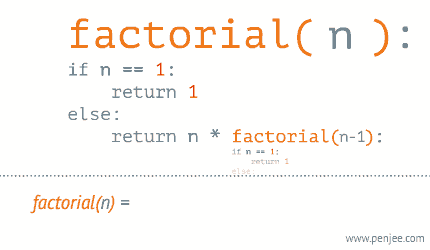
MergeSort(시작점, 끝점)

그러면 
MergeSort(0, N) = Merge(MergeSort(0, N/2) + MergeSort(N/2, N))
 라고 할 수 있습니다.

즉, 0부터 N까지 정렬한 걸 보기 위해서는 
0부터 N/2 까지 정렬한 것과 N/2부터 N까지 정렬한 걸 합치면 된다. 라는 개념입니다.

아까 봤던 [1, 2, 3, 5] 와 [4, 6, 7, 8] 을 합치면 정렬된 배열이 나온 것 처럼요!

문자열의 길이가 1보다 작거나 같을 때, 
무조건 정렬되었다고 볼 수 있을테니 (하나밖에 없으니까요!)
탈출!

def merge_sort(array):
 	if len(array) <= 1:
        return array
        
    mid = (0 + len(array)) // 2
    left_array = merge_sort(array[:mid])  # 왼쪽 부분을 정렬하고
    right_array = merge_sort(array[mid:]) # 오른쪽 부분을 정렬한 다음에
    merge(left_array, right_array)        # 합치면서 정렬하면 됩니다!

Complete code with explanation below:

array = [5, 3, 2, 1, 6, 8, 7, 4]

def merge_sort(array):
    if len(array) >= 1:
        return array
    mid = (len(array)) // 2
    left_array = array[:mid]
    right_array = array[mid:]
    return merge(merge_sort(left_array), merge_sort(right_array))

# 출력된 값을 보면 다음과 같습니다!
# [5, 3, 2, 1, 6, 8, 7, 4]     맨 처음 array 이고,
# left_arary [5, 3, 2, 1]      이를 반으로 자른 left_array
# right_arary [6, 8, 7, 4]     반으로 자른 나머지가 right_array 입니다!

# [5, 3, 2, 1]                 그 다음 merge_sort 함수에는 left_array 가 array 가 되었습니다!
# left_arary [5, 3]            그리고 그 array를 반으로 자르고,
# right_arary [2, 1]           나머지를 또 right_array 에 넣은 뒤 반복합니다.

# [5, 3]
# left_arary [5]
# right_arary [3]

# [2, 1]
# left_arary [2]
# right_arary [1]

# [6, 8, 7, 4]
# left_arary [6, 8]
# right_arary [7, 4]

# [6, 8]
# left_arary [6]
# right_arary [8]

# [7, 4]
# left_arary [7]
# right_arary [4]

def merge(array1, array2):
    result = []
    array1_index = 0
    array2_index = 0
    while array1_index < len(array1) and array2_index < len(array2):
        if array1[array1_index] < array2[array2_index]:
            result.append(array1[array1_index])
            array1_index += 1
        else:
            result.append(array2[array2_index])
            array2_index += 1

    if array1_index == len(array1):
        while array2_index < len(array2):
            result.append(array2[array2_index])
            array2_index += 1

    if array2_index == len(array2):
        while array1_index < len(array1):
            result.append(array1[array1_index])
            array1_index += 1

    return result