이전 시간에 배웠듯이 linear model은 오직 하나의 global optima를 가지므로,
linear model임이 확정된다면, 미분값 0인 지점을 단순 계산으로 찾아 J(β)가 최소인 지점을 정의하는 것이 가능하다!

🐱‍🏍 Normal Equations

As linear models always have a global optima (no local optima), we can use a nice way to get parameters without iterations.

✔ Derivation

이 두 장의 슬라이드는 잘 이해가 가지 않지만
어쩌겟습니까? 암튼 중요한 건 다음 부분임
(your brain power may be a burden)

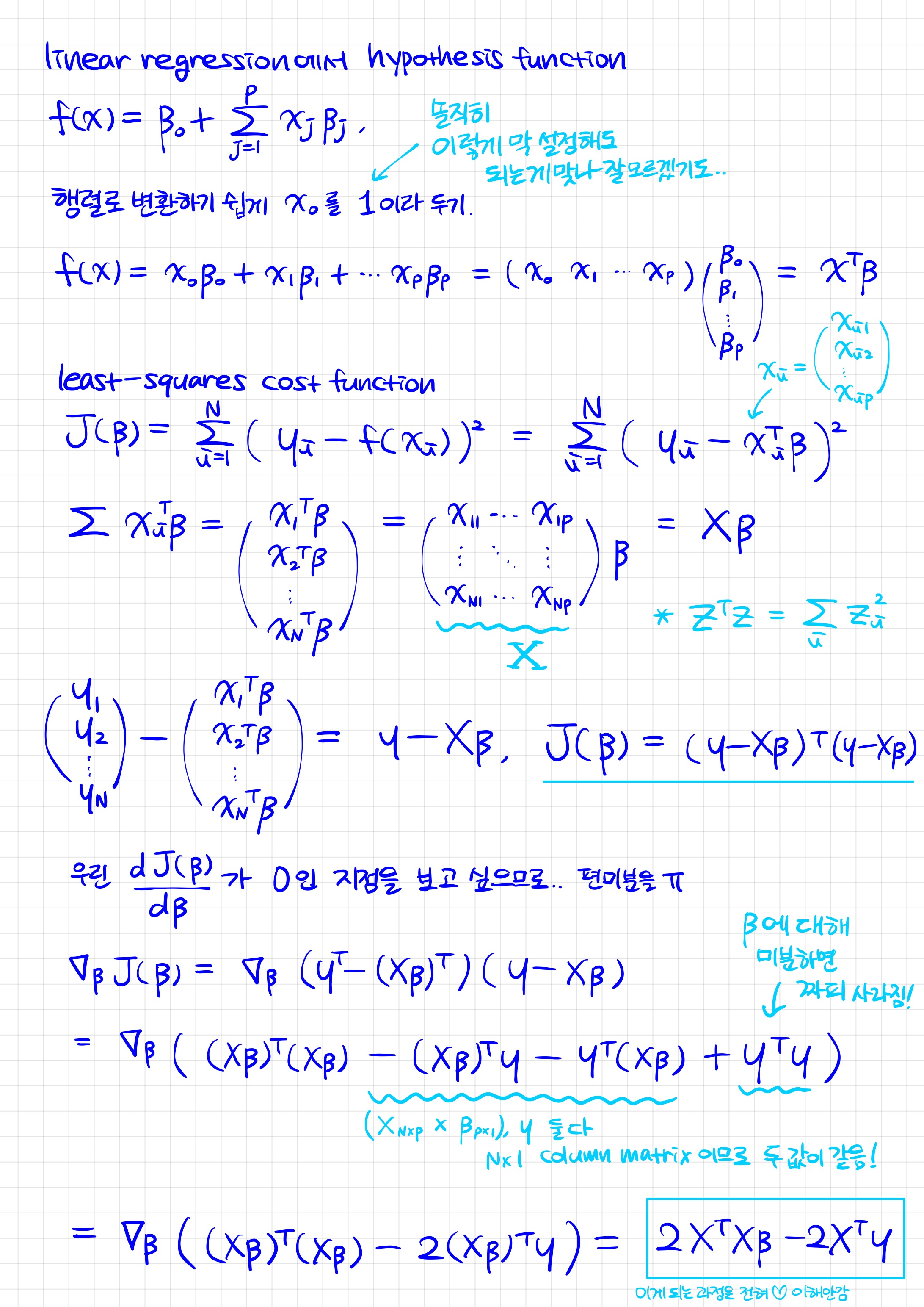
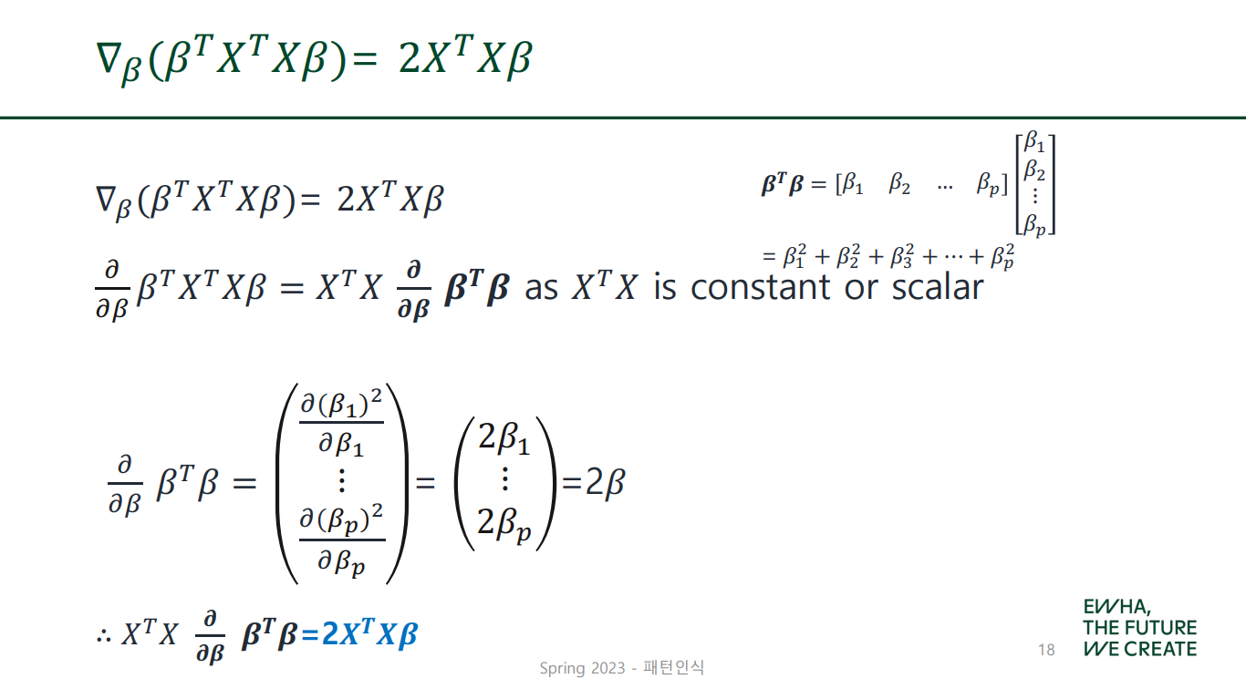
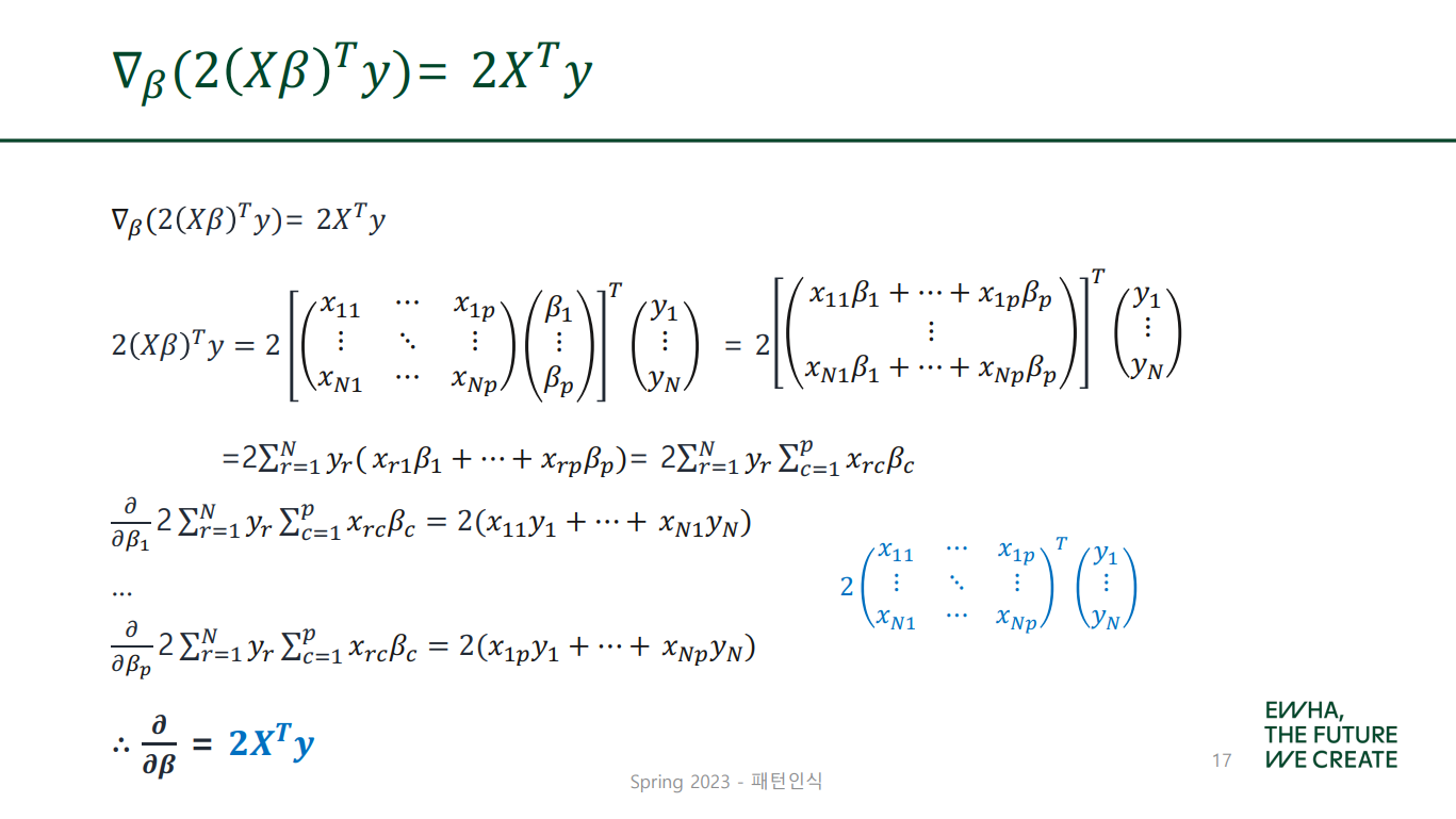
cost function J(β)를 β에 대해 미분한 값, 즉
$∇_βJ(β) = 2X^TXβ - 2X^Ty$임을 알았으며,
이 값이 0이 되는 β는 다음과 같이 찾을 수 있다!

$β = (X^TX)^{-1}X^Ty$

✔ Gradient Descent vs. Normal Equation

	Gradient Descent	Normal Equation
방식	iteration 사용	단순 $(X^TX)^{-1}X^Ty$ 계산
학습률	좋은 학습률을 찾아야 함	없어도 됨
feature 수	많으면 좋음	많으면 계산 어려움 (적어야 좋음)
non-invertible 여부	상관없음	$X^TX$가 invertible이어야 함

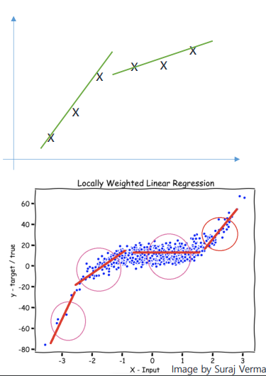
🐱‍🏍 Locally Weighted Linear Regression

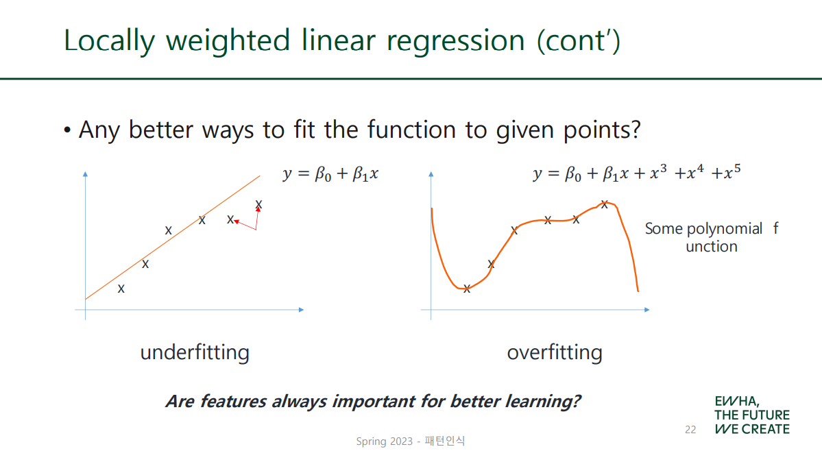
단순히 feature 수를 늘린다고 좋은 모델이 되는 것은 아님!
Overfitting의 위험이 존재하기 때문.

Overfitting

한마디로 학습 데이터에 대하여 과하게 학습한 나머지 실제 데이터에 대한 오차는 증가하는 현상! 노란 고양이 데이터로 고양이의 특성을 학습한 알고리즘이 하얀 고양이는 고양이로 인식하지 못하는 경우를 예로 들 수 있다.

그럼 feature 개수를 늘리는 것 말고
최적화를 위한 다른 방안은 없을까!?

✔ Cost Function in Locally Weighted Linear Regression

$J(β) = \displaystyle \sum^N_{i=1}w_i(y_i-x^T_iβ)^2$

$w_i$의 크기가...

• 작으면: negligible, error값을 작게 한다.
• 크면: makes the error shrinkage harder.

한글로 어케 번역해야 할지 모르겠지만
error값을 더 많이 반영하도록 한다 정도면 되지 않을까!

✔ Weight

가중치: 개별 구성요소가 차지하는 비중이나 중요도를 나타내는 수치

$w_i = \exp(-\displaystyle \frac {(x_i - x)^2}{2τ^2})$
$\therefore 0 < w_i ≤ 1$

아 exp란 거 이번에 처음 알았어... $\exp(-\displaystyle \frac {(x_i - x)^2}{2τ^2}) = e^{-\frac {(x_i - x)^2}{2τ^2}}$

1. If $x_i-x$ is...

• smaller: 가중치는 1에 가까워진다.
• bigger: 가중치는 0에 가까워진다.

2. $τ$ is... Bandwidth!

밴드 너비 고려할 이웃의 개수! $w_i$ 그래프의 폭 조정!

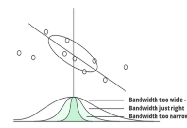
• smaller: 폭 좁아짐 (narrow) 적은 수의 이웃만 고려함.
• bigger: 폭 넓어짐 (wide) 많은 이웃을 고려함.

한마디로,

• $x_i$가 $x$로부터 멀리 떨어질수록 가중치 $w$는 0에 가까워지고, $x_i$의 error값은 무시해도 될 정도로 작은 값을 갖게 된다.
• 반대로 $x_i$가 $x$와 가까운 경우 가중치 $w$는 높은 값(1에 가까움)을 갖고, $x_i$의 error값은 중요하게 고려되는 것이다.

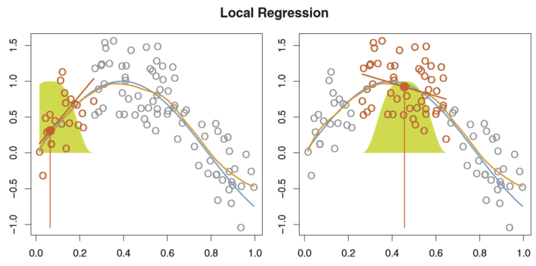
🐱‍🚀 그래프로 보기!

• 파란 그래프: represents $f(x)$ from which the data were generated

• 주황 그래프: corresponds to the local regression estimate

• 초록색 종 모양: indicates weights assigned to each point

• 주황색 점: the fitted value at $x_0$

• 주황색 선분 (기울기): the fit $f(x_0)$ at $x_0$ obtained by fitting a weighted linear regression

🐱‍🏍 Parametric vs. Non-parametric Algorithm

✔ Parametric model

The number of parameters is fixed! (The form of mapping function is defined before training starts)
ex) Linear regression, Logistic regression, Neural networks

• 모델의 파라미터 수가 정해져 있다.
• 특정한 데이터 분포를 따른다고 가정!
• 학습 속도가 상대적으로 빠르며, 모델을 이해하기 쉽다.

✔ Non-parametric model

The number of parameters can grow or shrink depending on the amount(size) of training data! (The form of mapping function is NOT defined)
ex) Locally weighted linear regression, Decision tree, random forest, k-NN

• 학습 데이터의 크기에 따라 파라미터 수가 달라진다.
• 데이터가 특정 분포를 따른다는 가정 X
• 상대적으로 flexible하며 데이터에 대한 사전 지식이 없을 때 유용하다.

---

참고자료

• https://www.datacamp.com/tutorial/tutorial-normal-equation-for-linear-regression
• https://towardsai.net/p/machine-learning/normal-equation-in-linear-regression
• https://math.stackexchange.com/questions/2133121/derivative-of-a-function-w-r-t-another-function
• https://blog.naver.com/je1206/220804412313
• https://towardsdatascience.com/locally-weighted-linear-regression-in-python-3d324108efbf
• https://xavierbourretsicotte.github.io/loess.html
• https://process-mining.tistory.com/131