DNN(심층 신경망) 응용예제

---

📦 MNIST 필기체 숫자 인식

import matplotlib.pyplot as plt
import tensorflow as tf

mnist = tf.keras.datasets.mnist
(x_train, y_train),(x_test, y_test) = mnist.load_data()
x_train, x_test = x_train / 255.0, x_test / 255.0

model = tf.keras.models.Sequential()
model.add(tf.keras.layers.Flatten(input_shape=(28,28)))
model.add(tf.keras.layers.Dense(512, activation='relu'))
model.add(tf.keras.layers.Dropout(0.2))
model.add(tf.keras.layers.Dense(10, activation='softmax'))

model.compile(optimizer='adam', loss='sparse_categorical_crossentropy', metrics=['accuracy'])
model.fit(x_train, y_train, epochs=5)
model.evaluate(x_test, y_test)

Epoch 1/5
60000/60000 [======================] - 7s 116us/sample - loss: 0.2205 - acc: 0.9348
Epoch 2/5
60000/60000 [======================] - 7s 110us/sample - loss: 0.0969 - acc: 0.9700
Epoch 3/5
60000/60000 [======================] - 7s 109us/sample - loss: 0.0678 - acc: 0.9785
Epoch 4/5
60000/60000 [======================] - 6s 108us/sample - loss: 0.0529 - acc: 0.9834
Epoch 5/5
60000/60000 [======================] - 7s 108us/sample - loss: 0.0428 - acc: 0.9859
10000/10000 [======================] - 0s 43us/sample - loss: 0.0645 - acc: 0.9795

---

📦 패션 아이템 분류

• 텐서플로우 튜토리얼에 나오는 패션 아이템을 심층 신경망으로 분류하는 코드

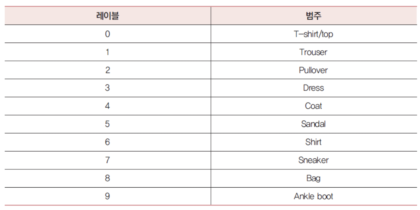
• 패션 MNIST 데이터셋은 10개의 범주(category)의 70,000개의 패션 관련 이미지 (옷, 구두, 핸드백 등)가 제공되며 해상도는 28x28이다.

• 이미지는 28x28 크기, 픽셀 값은 0과 255 사이

• 레이블(label)은 0에서 9까지의 정수로서 패션 아이템의 범주를 나타냄

import tensorflow as tf
from tensorflow import keras
import numpy as np
import matplotlib.pyplot as plt
from tensorflow.keras import datasets, layers, models

fashion_mnist = keras.datasets.fashion_mnist
(train_images, train_labels), (test_images, test_labels) = fashion_mnist.load_data()

plt.imshow(train_images[0])

train_images = train_images / 255.0
test_images = test_images / 255.0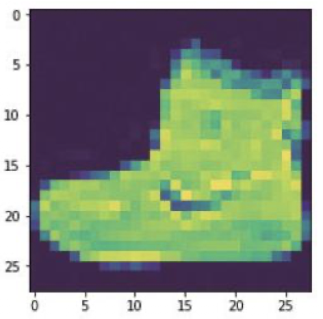

model = models.Sequential()
model.add(layers.Flatten(input_shape=(28, 28)))
model.add(layers.Dense(128, activation='relu'))
model.add(layers.Dense(10, activation='softmax'))

model.compile(optimizer='adam', loss='sparse_categorical_crossentropy', metrics=['accuracy'])

model.fit(train_images, train_labels, epochs=5)

test_loss, test_acc = model.evaluate(test_images, test_labels)
print('정확도:', test_acc)

10000/10000 [==============================] - 0s 32us/sample - loss: 0.3560 -
acc: 0.8701
정확도: 0.8701

---

📦 타이타닉 생존자 예측하기

• Kaggle 사이트에서 경진대회 참조 ("어떤 부류의 사람들의 생존률이 높았을까?" 에 대한 예측)

# 라이브러리 적재
import numpy as np
import matplotlib.pyplot as plt
import pandas as pd
import tensorflow as tf

# 학습 데이터 다운로드
# 타이타닉 데이터는 Kaggle 사이트(https://www.Kaggle.com/c/titanic/data)에서 다운로드 받는다.
# 학습데이터는 train.csv파일이고 테스트 데이터는 test.csv파일이다.

# 데이터 세트를 읽어들인다.
train = pd.read_csv("train.csv", sep=',')
test = pd.read_csv("test.csv", sep=',')

# 필요없는 컬럼을 삭제한다.
train.drop(['SibSp', 'Parch', 'Ticket', 'Embarked', 'Name', 'Cabin', 'PassengerId', 'Fare', 'Age'], inplace=True, axis=1)

# 결손치가 있는 데이터 행은 삭제한다.
train.dropna(inplace=True)

# 구글 드라이브 연결
from google.colab import drive
drive.mount('/content/drive')
# Mounted at /content/drive
import os
print(os.listdir('/content/drive/MyDrive'))
# ['Colab Notebooks', 'Google Form’,…]

# 성별에 따른 생존률 시각화
df = train.groupby('Sex').mean()["Survived"]
df.plot(kind='bar')
plt.show()

# Pcalss에 대해서도 생존률 그래프를 그려보면 상당한 인과관계가 있다는 것을 알 수 있다.
#따라서 학습의 입력으로 “Sex”와 “Pclass”만을 고려한다.

여성의 생존률이 높은 것을 알 수 있음

# 학습 데이터 정제
# train.drop(['SibSp', 'Parch', 'Ticket', 'Embarked', 'Name', 'Cabin', 'PassengerId', 'Fare', 'Age'], inplace=True, axis=1)
# inplace=True는 원래 데이터 프레임을 변경하라는 의미이고 axis=1은 축번호 1번 (즉 column)을 삭제하라는 의미이다.

train.head()
# Survived Pclass Sex
# 0 0 3 male
# 1 1 1 female
# 2 1 3 female
# 3 1 1 female
# 4 0 3 male

# 성별 기호를 수치로 변환한다.
# 딥러닝은 0부터 1사이의 실수만 처리 가능
for ix in train.index:
	if train.loc[ix, 'Sex']=="male":
		train.loc[ix, 'Sex']=1
	else:
		train.loc[ix, 'Sex']=0

# 2차원 배열을 1차원 배열로 평탄화한다.
target = np.ravel(train.Survived)

# 생존여부를 학습 데이터에서 삭제한다.
train.drop(['Survived'], inplace=True, axis=1)
train = train.astype(float) # 최근 소스에서는 float형태로 형변환하여야 한다.

# 케라스 모델을 생성한다.
model = tf.keras.models.Sequential()
model.add(tf.keras.layers.Dense(16, activation='relu', input_shape=(2,)))
model.add(tf.keras.layers.Dense(8, activation='relu'))
model.add(tf.keras.layers.Dense(1, activation='sigmoid'))

# 케라스 모델을 컴파일한다.
model.compile(loss='binary_crossentropy', optimizer='adam', metrics=['accuracy'])

# 케라스 모델을 학습시킨다.
model.fit(train, target, epochs=30, batch_size=1, verbose=1)

...
Epoch 29/30
891/891 [==============================] - 1s 753us/sample - loss: 0.4591 - acc: 0.7677
Epoch 30/30
891/891 [==============================] - 1s 753us/sample - loss: 0.4547 - acc: 0.7789