Variational Autoencoder

1. Settings

1) Import required libraries

import numpy as np
import torch
import torch.nn as nn
import torch.optim as optim
import torch.nn.init as init
import torchvision.datasets as dset
import torchvision.transforms as transforms
from torch.utils.data import DataLoader
from torchvision.utils import make_grid # It helps us make grid style figures form like multiple images
import matplotlib.pyplot as plt
import matplotlib as mpl
from IPython.display import Image

2) Set hyperparameters

batch_size = 128
learning_rate = 1e-3
num_epochs = 10

2. Data

1) Download Data

mnist_train = dset.MNIST("./", train=True, transform=transforms.ToTensor(), target_transform=None, download=True)
mnist_test = dset.MNIST("./", train=False, transform=transforms.ToTensor(), target_transform=None, download=True)
mnist_train, mnist_val = torch.utils.data.random_split(mnist_train, [50000, 10000])
# 따로 augmentation은 안하고 image를 tensor form으로 바꾸기만 하였다.

Downloading http://yann.lecun.com/exdb/mnist/train-images-idx3-ubyte.gz
Downloading http://yann.lecun.com/exdb/mnist/train-images-idx3-ubyte.gz to ./MNIST/raw/train-images-idx3-ubyte.gz



  0%|          | 0/9912422 [00:00<?, ?it/s]


Extracting ./MNIST/raw/train-images-idx3-ubyte.gz to ./MNIST/raw

Downloading http://yann.lecun.com/exdb/mnist/train-labels-idx1-ubyte.gz
Downloading http://yann.lecun.com/exdb/mnist/train-labels-idx1-ubyte.gz to ./MNIST/raw/train-labels-idx1-ubyte.gz



  0%|          | 0/28881 [00:00<?, ?it/s]


Extracting ./MNIST/raw/train-labels-idx1-ubyte.gz to ./MNIST/raw

Downloading http://yann.lecun.com/exdb/mnist/t10k-images-idx3-ubyte.gz
Downloading http://yann.lecun.com/exdb/mnist/t10k-images-idx3-ubyte.gz to ./MNIST/raw/t10k-images-idx3-ubyte.gz



  0%|          | 0/1648877 [00:00<?, ?it/s]


Extracting ./MNIST/raw/t10k-images-idx3-ubyte.gz to ./MNIST/raw

Downloading http://yann.lecun.com/exdb/mnist/t10k-labels-idx1-ubyte.gz
Downloading http://yann.lecun.com/exdb/mnist/t10k-labels-idx1-ubyte.gz to ./MNIST/raw/t10k-labels-idx1-ubyte.gz



  0%|          | 0/4542 [00:00<?, ?it/s]


Extracting ./MNIST/raw/t10k-labels-idx1-ubyte.gz to ./MNIST/raw

mnist_train[0][0].size()    # (1, 28, 28)

torch.Size([1, 28, 28])

mnist_train[0][1]           # label

2

2) Set DataLoader

dataloaders = {}
dataloaders['train'] = DataLoader(mnist_train, batch_size=batch_size, shuffle=True)
dataloaders['val'] = DataLoader(mnist_val, batch_size=batch_size, shuffle=False)
dataloaders['test'] = DataLoader(mnist_test, batch_size=batch_size, shuffle=False)

len(dataloaders["train"])

391

3. Model & Optimizer

# https://lilianweng.github.io/lil-log/2018/08/12/from-autoencoder-to-beta-vae.html
!wget -q https://www.dropbox.com/s/lmpjzzkqhk7d408/vae_gaussian.png
Image("vae_gaussian.png")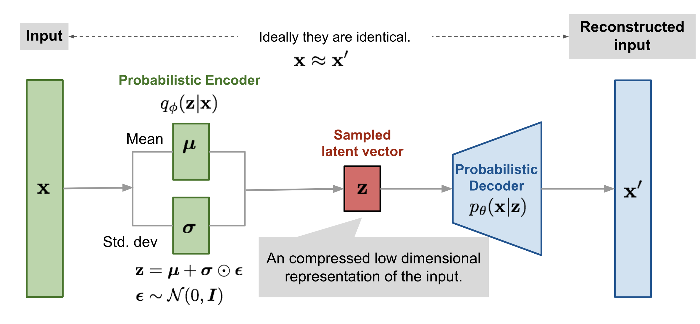

1) Model

# build your own variational autoencoder
# encoder: 784(28*28) -> 256
# sampling: 256 -> 10
# decoder: 10 -> 256 -> 784(28*28)

class VariationalAutoencoder(nn.Module):
    def __init__(self):
        super(VariationalAutoencoder,self).__init__()
        self.encoder = nn.Sequential(
            nn.Linear(28*28, 256),    
            nn.Tanh(),                          # activation function
        )
        
        self.fc_mu = nn.Linear(256, 10)
        self.fc_var = nn.Linear(256, 10)
        
        self.decoder = nn.Sequential(
            nn.Linear(10, 256),
            nn.Tanh(),                          # activation function
            nn.Linear(256, 28*28),
            nn.Sigmoid()
        )
                
    def encode(self, x):
        h = self.encoder(x)
        mu = self.fc_mu(h)
        log_var = self.fc_var(h)
        return mu, log_var
    
    def reparameterize(self, mu, log_var):
        std = torch.exp(0.5*log_var)
        # randn_like : make gaussian distribution and make same size with target tensor
        eps = torch.randn_like(std)
        return mu + eps*std
    
    def decode(self, z):
        recon = self.decoder(z)
        return recon
    
                
    def forward(self, x):                # x: (batch_size, 1, 28, 28)
        batch_size = x.size(0)
        mu, log_var = self.encode(x.view(batch_size, -1))
        z = self.reparameterize(mu, log_var)
        out = self.decode(z)
        return out, mu, log_var

2) Loss func & Optimizer

device = torch.device("cuda:0" if torch.cuda.is_available() else "cpu")
print(device)

cuda:0

BCE = torch.nn.BCELoss(reduction='sum')

def loss_func(x, recon_x, mu, log_var):
    #batch_size = x.size(0)
    #MSE_loss = MSE(x, recon_x.view(batch_size, 1, 28, 28))

    BCE_loss = BCE(recon_x, x.view(-1, 784))
    KLD_loss = -0.5 * torch.sum(1 + log_var - mu.pow(2) - log_var.exp())
    return BCE_loss + KLD_loss

model = VariationalAutoencoder().to(device)
optimizer = torch.optim.Adam(model.parameters(), lr=learning_rate)

4. Train

import time
import copy

def train_model(model, dataloaders, criterion, optimizer, num_epochs=10):
    """
    model: model to train
    dataloaders: train, val, test data's loader
    criterion: loss function
    optimizer: optimizer to update your model
    """
    since = time.time()

    train_loss_history = []
    val_loss_history = []

    best_model_wts = copy.deepcopy(model.state_dict())
    best_val_loss = 100000000

    for epoch in range(num_epochs):
        print('Epoch {}/{}'.format(epoch, num_epochs - 1))
        print('-' * 10)

        # Each epoch has a training and validation phase
        for phase in ['train', 'val']:
            if phase == 'train':
                model.train()            # Set model to training mode
            else:
                model.eval()            # Set model to evaluate mode

            running_loss = 0.0

            # Iterate over data.
            for inputs, labels in dataloaders[phase]:
                inputs = inputs.to(device)                                       # transfer inputs to GPU 

                # zero the parameter gradients
                optimizer.zero_grad()

                # forward
                # track history if only in train
                with torch.set_grad_enabled(phase == 'train'):

                    outputs, mu, log_var = model(inputs)
                    loss = criterion(inputs, outputs, mu, log_var)  # calculate a loss


                    # backward + optimize only if in training phase
                    if phase == 'train':
                        loss.backward()                             # perform back-propagation from the loss
                        optimizer.step()                             # perform gradient descent with given optimizer

                # statistics
                running_loss += loss.item()

            epoch_loss = running_loss / len(dataloaders[phase].dataset)

            print('{} Loss: {:.4f}'.format(phase, epoch_loss))
            
            # deep copy the model
            if phase == 'train':
                train_loss_history.append(epoch_loss)

            if phase == 'val':
                val_loss_history.append(epoch_loss)

            if phase == 'val' and epoch_loss < best_val_loss:
                best_val_loss = epoch_loss
                best_model_wts = copy.deepcopy(model.state_dict())
            

        print()

    time_elapsed = time.time() - since
    print('Training complete in {:.0f}m {:.0f}s'.format(time_elapsed // 60, time_elapsed % 60))
    print('Best val Loss: {:4f}'.format(best_val_loss))

    # load best model weights
    model.load_state_dict(best_model_wts)
    return model, train_loss_history, val_loss_history

best_model, train_loss_history, val_loss_history = train_model(model, dataloaders, loss_func, optimizer, num_epochs=num_epochs)

Epoch 0/9
----------
train Loss: 176.3736
val Loss: 143.7017

Epoch 1/9
----------
train Loss: 139.2582
val Loss: 136.5507

Epoch 2/9
----------
train Loss: 132.6491
val Loss: 130.2981

Epoch 3/9
----------
train Loss: 128.1843
val Loss: 126.5062

Epoch 4/9
----------
train Loss: 124.9720
val Loss: 123.9947

Epoch 5/9
----------
train Loss: 122.4792
val Loss: 122.2747

Epoch 6/9
----------
train Loss: 120.4484
val Loss: 120.0995

Epoch 7/9
----------
train Loss: 118.9096
val Loss: 118.8826

Epoch 8/9
----------
train Loss: 117.5928
val Loss: 117.9884

Epoch 9/9
----------
train Loss: 116.5053
val Loss: 116.5101

Training complete in 1m 23s
Best val Loss: 116.510067

# Let's draw a learning curve like below.
plt.plot(train_loss_history, label='train')
plt.plot(val_loss_history, label='val')
plt.xlabel('epoch')
plt.ylabel('loss')
plt.legend()
plt.show()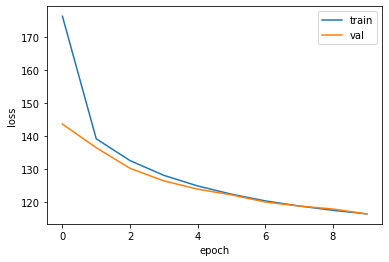

5. Check with Test Image (Can VAE reconstruct input images?)

with torch.no_grad():
    running_loss = 0.0
    for inputs, labels in dataloaders["test"]:
        inputs = inputs.to(device)

        outputs, mu, log_var = best_model(inputs)
        test_loss = loss_func(inputs, outputs, mu, log_var)
        
        running_loss += test_loss.item()

    test_loss = running_loss / len(dataloaders["test"].dataset)
    print(test_loss)        

115.27722764892579

out_img = torch.squeeze(outputs.cpu().data)
print(out_img.size())

for i in range(5):
    plt.subplot(1,2,1)
    plt.imshow(torch.squeeze(inputs[i]).cpu().numpy(),cmap='gray')
    plt.subplot(1,2,2)
    plt.imshow(out_img[i].numpy().reshape(28, 28),cmap='gray')
    plt.show()

torch.Size([16, 784])

6. Visualizing MNIST

np.random.seed(42)

from sklearn.manifold import TSNE

train_dataset_array = mnist_train.dataset.data.numpy() / 255
train_dataset_array = np.float32(train_dataset_array)
labels = mnist_train.dataset.targets.numpy()

subset_indices = []
subset_indices_per_class = []

for i in range(10):
    indices = np.where(labels == i)[0]
    subset_size = len(indices) // 6
    subset_indices += indices[:subset_size].tolist()
    subset_indices_per_class.append(indices[:subset_size].tolist())

train_dataset_array = train_dataset_array[subset_indices]
labels = labels[subset_indices]

train_dataset_array = torch.tensor(train_dataset_array)
inputs = train_dataset_array.to(device)
outputs, mu, log_var = best_model(inputs)

encoded = mu.cpu().detach().numpy()
tsne = TSNE()   
X_train_2D = tsne.fit_transform(encoded)
X_train_2D = (X_train_2D - X_train_2D.min()) / (X_train_2D.max() - X_train_2D.min())

plt.scatter(X_train_2D[:, 0], X_train_2D[:, 1], c=labels, s=10, cmap="tab10")
plt.axis("off")
plt.show()

Let's make this diagram a bit prettier:

# adapted from https://scikit-learn.org/stable/auto_examples/manifold/plot_lle_digits.html
plt.figure(figsize=(10, 8))
cmap = plt.cm.tab10
plt.scatter(X_train_2D[:, 0], X_train_2D[:, 1], c=labels, s=10, cmap=cmap)
image_positions = np.array([[1., 1.]])
for index, position in enumerate(X_train_2D):
    dist = np.sum((position - image_positions) ** 2, axis=1)
    if np.min(dist) > 0.02: # if far enough from other images
        image_positions = np.r_[image_positions, [position]]
        imagebox = mpl.offsetbox.AnnotationBbox(
            mpl.offsetbox.OffsetImage(torch.squeeze(inputs).cpu().numpy()[index], cmap="binary"),
            position, bboxprops={"edgecolor": cmap(labels[index]), "lw": 2})
        plt.gca().add_artist(imagebox)
plt.axis("off")
plt.show()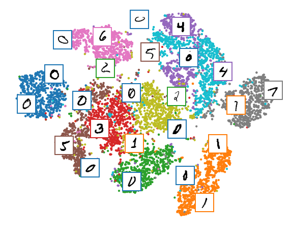

7. Walk through latent space of MNIST

encoded.shape

(9996, 10)

mean_encoded = []
for i in range(10):
    mean_encoded.append(encoded[np.where(labels == i)[0]].mean(axis=0))

selected_class = [1, 7]
samples = []
with torch.no_grad():
    for idx, coef in enumerate(np.linspace(0, 1, 10)):
        interpolated = coef * mean_encoded[selected_class[0]] + (1.-coef) * mean_encoded[selected_class[1]]
        samples.append(interpolated)
    samples = np.stack(samples)
    z = torch.tensor(samples).to(device)
    generated = best_model.decoder(z).to(device)

generated = generated.view(10, 1, 28, 28)
img = make_grid(generated, nrow=10)
npimg = img.cpu().numpy()
plt.imshow(np.transpose(npimg, (1,2,0)), interpolation='nearest')

<matplotlib.image.AxesImage at 0x7f5e6d257070>

selected_class = [1, 8]
samples = []
with torch.no_grad():
    for idx, coef in enumerate(np.linspace(0, 1, 10)):
        interpolated = coef * mean_encoded[selected_class[0]] + (1.-coef) * mean_encoded[selected_class[1]]
        samples.append(interpolated)
    samples = np.stack(samples)
    z = torch.tensor(samples).to(device)
    generated = best_model.decoder(z).to(device)

generated = generated.view(10, 1, 28, 28)
img = make_grid(generated, nrow=10)
npimg = img.cpu().numpy()
plt.imshow(np.transpose(npimg, (1,2,0)), interpolation='nearest')

<matplotlib.image.AxesImage at 0x7f5e6d22cdc0>

selected_class = [6, 8]
samples = []
with torch.no_grad():
    for idx, coef in enumerate(np.linspace(0, 1, 10)):
        interpolated = coef * mean_encoded[selected_class[0]] + (1.-coef) * mean_encoded[selected_class[1]]
        samples.append(interpolated)
    samples = np.stack(samples)
    z = torch.tensor(samples).to(device)
    generated = best_model.decoder(z).to(device)

generated = generated.view(10, 1, 28, 28)
img = make_grid(generated, nrow=10)
npimg = img.cpu().numpy()
plt.imshow(np.transpose(npimg, (1,2,0)), interpolation='nearest')

<matplotlib.image.AxesImage at 0x7f5e6d189b80>

8. Comparison between low capacity model and high capacity model

# build your own variational autoencoder
# encoder: 784(28*28) -> 512 -> 256
# sampling: 256 -> 10
# decoder: 10 -> 256 -> 512 -> 784(28*28)

class VariationalAutoencoderHigh(nn.Module):
    def __init__(self):
        super(VariationalAutoencoderHigh,self).__init__()
        self.encoder = nn.Sequential(
            nn.Linear(28*28, 512),    
            nn.ReLU(),                          # activation function
            nn.Linear(512, 256),
            nn.ReLU()                           # activation function
        )
        
        self.fc_mu = nn.Linear(256, 10)
        self.fc_var = nn.Linear(256, 10)
        
        self.decoder = nn.Sequential(
            nn.Linear(10, 256),
            nn.ReLU(),                          # activation function
            nn.Linear(256, 512),
            nn.ReLU(),                          # activation function
            nn.Linear(512, 28*28),
            nn.Sigmoid()
        )
                
    def encode(self, x):
        h = self.encoder(x)
        mu = self.fc_mu(h)
        log_var = self.fc_var(h)
        return mu, log_var
    
    def reparameterize(self, mu, log_var):
        std = torch.exp(0.5*log_var)
        eps = torch.randn_like(std)
        return mu + eps*std
    
    def decode(self, z):
        recon = self.decoder(z)
        return recon
    
                
    def forward(self, x):                # x: (batch_size, 1, 28, 28)
        batch_size = x.size(0)
        mu, log_var = self.encode(x.view(batch_size, -1))
        z = self.reparameterize(mu, log_var)
        out = self.decode(z)
        return out, mu, log_var

model = VariationalAutoencoderHigh().to(device)
optimizer = torch.optim.Adam(model.parameters(), lr=learning_rate)

best_model_high, train_loss_history_high, val_loss_history_high = train_model(model, dataloaders, loss_func, optimizer, num_epochs=num_epochs)

Epoch 0/9
----------
train Loss: 177.1977
val Loss: 138.0068

Epoch 1/9
----------
train Loss: 129.4368
val Loss: 124.0840

Epoch 2/9
----------
train Loss: 120.4661
val Loss: 118.0296

Epoch 3/9
----------
train Loss: 115.4424
val Loss: 114.2469

Epoch 4/9
----------
train Loss: 112.5352
val Loss: 111.9914

Epoch 5/9
----------
train Loss: 110.7230
val Loss: 110.7401

Epoch 6/9
----------
train Loss: 109.1535
val Loss: 109.1290

Epoch 7/9
----------
train Loss: 107.6706
val Loss: 108.4114

Epoch 8/9
----------
train Loss: 106.6582
val Loss: 107.0636

Epoch 9/9
----------
train Loss: 105.7405
val Loss: 106.4770

Training complete in 1m 25s
Best val Loss: 106.476992

# Let's draw a learning curve for low and high capacity models.
plt.plot(train_loss_history, label='low_train')
plt.plot(val_loss_history, label='low_val')
plt.plot(train_loss_history_high, label='high_train')
plt.plot(val_loss_history_high, label='high_val')
plt.xlabel('epoch')
plt.ylabel('loss')
plt.legend()
plt.show()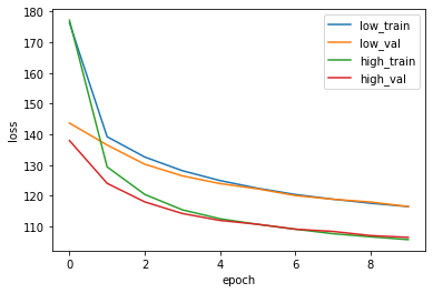

with torch.no_grad():
    running_loss = 0.0
    for inputs, labels in dataloaders["test"]:
        inputs = inputs.to(device)

        outputs, mu, log_var = best_model_high(inputs) # best_model_high 
        test_loss = loss_func(inputs, outputs, mu, log_var)
        
        running_loss += test_loss.item()

    test_loss = running_loss / len(dataloaders["test"].dataset)
    print(test_loss)        

105.40507999267578

out_img_high = torch.squeeze(outputs.cpu().data) # out_img_high
print(out_img.size())

for i in range(5):
    plt.subplot(1,3,1)
    plt.imshow(torch.squeeze(inputs[i]).cpu().numpy(),cmap='gray')
    plt.subplot(1,3,2)
    plt.imshow(out_img[i].numpy().reshape(28, 28),cmap='gray')
    plt.subplot(1,3,3)
    plt.imshow(out_img_high[i].numpy().reshape(28, 28),cmap='gray')
    plt.show()

torch.Size([16, 784])

9. BCE loss and MSE loss

#Tutorial on Variational Autoencoders Carl Doersch
!wget -q https://www.dropbox.com/s/5kkhyo7apxkay5z/BCE_loss%20and%20MSE_loss.PNG
Image("BCE_loss and MSE_loss.PNG")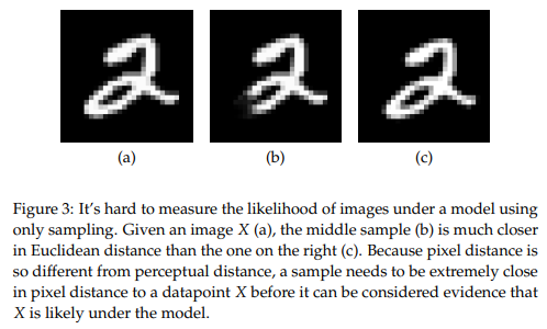

(a) : original image
(b) and (c) : reconstructive image

Difference between BCE loss and MSE loss
If you use BCE loss, it will get classification loss. So the model will take semantic meaning of MNIST image not just pixel to pixel comparison like MSE loss.

(b)는 (a)에서 일부분을 지운 것이고, (c)는 (a)를 shift한 것이다.
MSE loss를 사용하면 (a)와 (b)의 loss가 (a)와 (c)의 loss보다 작다. Pixel comparison을 하기 때문!
하지만 BCE loss를 사용하면 (a)와 (c)의 loss가 (a)와 (b)의 loss보다 작다. Semantic meaning을 학습하려고 하기 때문!

Reference

• AI504: Programming for AI Lecture at KAIST AI