토픽 모델링
1) 잠재 의미 분석(Latent Semantic Analysis, LSA)
LSA는 토픽 모델링을 위한 아이디어를 제공했음. LDA가 LSA를 개선해 토픽 모델링에 좀 더 최적화
DTM과 TF-IDF는 빈도 기반 수치화 방법이기 때문에 단어 의미를 고려하지 못하는 한계가 있었음. Latent(잠재된) 의미를 이끌어내는 방법이 LSA. 이를 이해하기 위해선 SVD(특이값 분해)를 알아야 함.
1. 특이값 분해(Singular Value Decomposition)
SVD란 A가 m x n일 때 , 3개의 행렬 곱으로 decomposition!
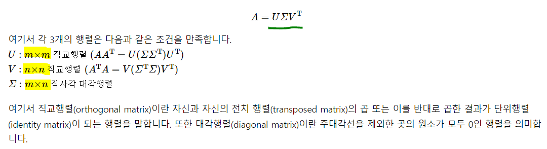
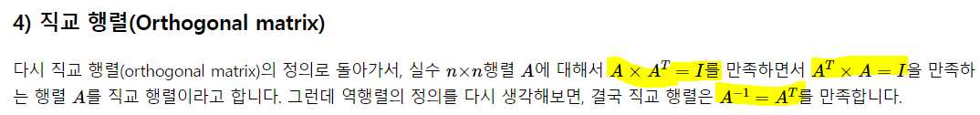
A의 전치가 역행렬일 때 이를 Orthogonal!
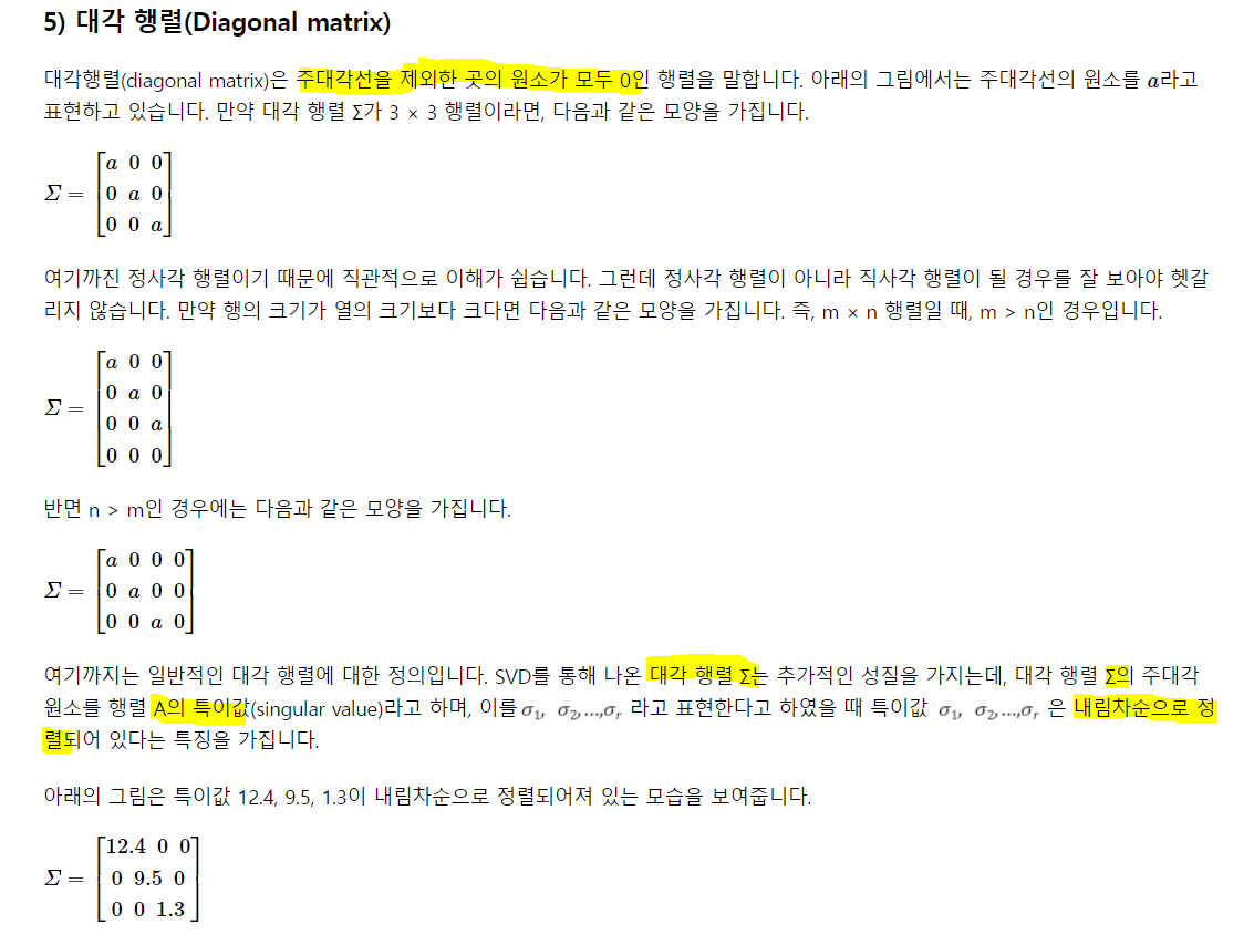
시그마 안에 특이값들이 들어있고, 내림차순으로 정렬.
3. 잠재 의미 분석
DTM이나 TF-IDF는 단어 의미를 고려하지 못한다는 단점이 존재. LSA는 기본적으로 이 행렬을 활용해 절단된 SVD를 사용해 차원을 축소시키고 잠재적인 의미를 끌어낸다는 아이디어를 가짐.
이 DTM을 이용!
import numpy as np
A=np.array([[0,0,0,1,0,1,1,0,0],[0,0,0,1,1,0,1,0,0],[0,1,1,0,2,0,0,0,0],[1,0,0,0,0,0,0,1,1]])
np.shape(A)
(4, 9)4행 9열짜리 matrix가 생성.
풀 SVD를 진행, 시그마 대신 S로, t(V) 대신 VT로 표현
U, s, VT = np.linalg.svd(A, full_matrices = True)
print(U.round(2))
np.shape(U)
[[-0.24 0.75 0. -0.62]
[-0.51 0.44 -0. 0.74]
[-0.83 -0.49 -0. -0.27]
[-0. -0. 1. 0. ]]
(4, 4)U의 shape을 봤고, U는 A가 m x n 행렬일 때 m x m 의 shape을 가짐
np.linalg.inv(U), np.transpose(U)(array([[-2.39751712e-01, -5.06077194e-01, -8.28495619e-01,
-8.78352025e-17],
[ 7.51083898e-01, 4.44029376e-01, -4.88580485e-01,
-2.98807451e-17],
[ 9.90665210e-17, -1.48599782e-16, -4.39152715e-17,
1.00000000e+00],
[-6.15135834e-01, 7.39407727e-01, -2.73649629e-01,
1.58797796e-16]]),
array([[-2.39751712e-01, -5.06077194e-01, -8.28495619e-01,
-8.78352025e-17],
[ 7.51083898e-01, 4.44029376e-01, -4.88580485e-01,
-2.98807451e-17],
[ 9.90665210e-17, -1.48599782e-16, -4.39152715e-17,
1.00000000e+00],
[-6.15135834e-01, 7.39407727e-01, -2.73649629e-01,
1.58797796e-16]])) U의 inverse와 transpose를 보면 그 값이 같음을 알 수 있다. Orthogonal 이므로.
numpy의 linalg.svd는 특이값을 행렬이 아니라 특이값 리스트를 반환한다. 따라서 특이값을 원소로 갖는 대각행렬을 생성해줘야 함. shape == (m, n)
S = np.zeros((4, 9))
S[:4, :4] = np.diag(s)
print(S.round(2))
S.shape
[[2.69 0. 0. 0. 0. 0. 0. 0. 0. ]
[0. 2.05 0. 0. 0. 0. 0. 0. 0. ]
[0. 0. 1.73 0. 0. 0. 0. 0. 0. ]
[0. 0. 0. 0.77 0. 0. 0. 0. 0. ]]
(4, 9)특이값 행렬로 변환해 줌. m x n shape
print(VT.round(2))
VT.shape
[[-0. -0.31 -0.31 -0.28 -0.8 -0.09 -0.28 -0. -0. ]
[ 0. -0.24 -0.24 0.58 -0.26 0.37 0.58 -0. -0. ]
[ 0.58 -0. 0. 0. -0. 0. -0. 0.58 0.58]
[ 0. -0.35 -0.35 0.16 0.25 -0.8 0.16 -0. -0. ]
[-0. -0.78 -0.01 -0.2 0.4 0.4 -0.2 0. 0. ]
[-0.29 0.31 -0.78 -0.24 0.23 0.23 0.01 0.14 0.14]
[-0.29 -0.1 0.26 -0.59 -0.08 -0.08 0.66 0.14 0.14]
[-0.5 -0.06 0.15 0.24 -0.05 -0.05 -0.19 0.75 -0.25]
[-0.5 -0.06 0.15 0.24 -0.05 -0.05 -0.19 -0.25 0.75]]
(9, 9)t(V)는 위와 같음. shape은 n x n 이므로 9 x 9.
np.allclose(A, np.dot(np.dot(U, S), VT).round(2))Truenp.allclose는 두 행렬이 동일하면 True를 리턴. A = USVT 임을 증명.
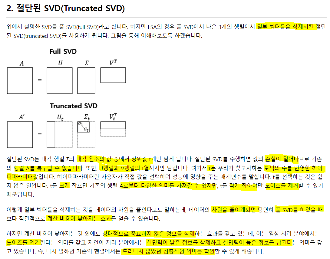
지금까진, 풀 SVD를 했고 원래 목적인 truncated SVD를 수행.
## 상위 두 개의 특이값만 남겨 둠.
S = S[:2, :2]
U = U[:, :2]
VT = VT[:2, :]
A_prime = np.dot(np.dot(U, S), VT)
print(A)
print(A_prime.round(2))
[[0 0 0 1 0 1 1 0 0]
[0 0 0 1 1 0 1 0 0]
[0 1 1 0 2 0 0 0 0]
[1 0 0 0 0 0 0 1 1]]
[[ 0. -0.17 -0.17 1.08 0.12 0.62 1.08 -0. -0. ]
[ 0. 0.2 0.2 0.91 0.86 0.45 0.91 0. 0. ]
[ 0. 0.93 0.93 0.03 2.05 -0.17 0.03 0. 0. ]
[ 0. 0. 0. 0. 0. -0. 0. 0. 0. ]] A와 truncated SVD를 통해 만든 A와 비교한 결과이다.
기존에 0을 가지던 것들은 대체적으로 가까운 값을 가짐.
축소된 U는 4 x 2의 크기를 가지는데, 이는 문서의 개수 * 토픽 t의 크기. 총 단어의 수는 9지만 토픽은 2로 표현. U의 각 행은 잠재 의미를 표현하기 위한 수치화 된 각각의 문서 벡터라고 볼 수 있음.
VT는 2 x 9의 크기로, 토픽의 수 X 단어의 수. 각 열은 잠재 의미를 표현하기 위해 수치화된 각각의 단어 벡터라고 볼 수 있음.
4. 실습을 통한 이해
사이킷런에 Twenty Newsgroups라는 20개의 다른 주제를 가진 뉴스그룹 데이터를 제공. LSA가 토픽 모델링에 최저은 아니지만, 시초가 되므로 LSA를 사용해서 토픽 모델링을 진행. t개의 토픽으로 압축하고, 각 토픽당 가장 중요한 단어 5개를 출력해보는 식으로 진행
import pandas as pd
from sklearn.datasets import fetch_20newsgroups
## 제거할 건 제거하고 랜덤하게 생성
dataset = fetch_20newsgroups(shuffle = True, random_state = 1, remove = ['headers', 'footers', 'quotes'])
documents = dataset.data
len(documents)11314총 11314개. 이 중 첫번 째 확인
documents[1]'\n\n\n\n\n\n\nYeah, do you expect people to read the FAQ, etc. and actually accept hard\natheism? No, you need a little leap of faith, Jimmy. Your logic runs out\nof steam!\n\n\n\n\n\n\n\nJim,\n\nSorry I can't pity you, Jim. And I'm sorry that you have these feelings of\ndenial about the faith you need to get by. Oh well, just pretend that it will\nall end happily ever after anyway. Maybe if you start a new newsgroup,\nalt.atheist.hard, you won't be bummin' so much?\n\n\n\n\n\n\nBye-Bye, Big Jim. Don't forget your Flintstone's Chewables! :) \n--\nBake Timmons, III'특수문자가 포함된 영어 문장으로 구서오디어 있음. 이런 형식이 11314개 존재. target_name을 보면 뉴스그룹 데이터가 어떤 20개의 카테고리를 갖고 있었는지 저장
dataset.target_names['alt.atheism',
'comp.graphics',
'comp.os.ms-windows.misc',
'comp.sys.ibm.pc.hardware',
'comp.sys.mac.hardware',
'comp.windows.x',
'misc.forsale',
'rec.autos',
'rec.motorcycles',
'rec.sport.baseball',
'rec.sport.hockey',
'sci.crypt',
'sci.electronics',
'sci.med',
'sci.space',
'soc.religion.christian',
'talk.politics.guns',
'talk.politics.mideast',
'talk.politics.misc',
'talk.religion.misc']2) 텍스트 전처리
기본적으로 정제를 거쳐야 함. 알파벳을 제외한 구두점, 숫자, 특수문저만 제거. 또한, 짧은 단어는 유용한 정보가 없다 생각해 제외하고, 모든 알파벳을 소문자로 바꿔 단어의 개수를 줄여주는 식으로 진행.
## df로 변환
news_df = pd.DataFrame({'document': documents})
# 특수문자 제거
news_df['clean_doc'] = news_df.document.str.replace('[^a-zA-Z]', ' ')
# 길이가 3이하는 제거
# 띄어쓰기 기준으로 분리하고 단어가 3글자 이하는 제거하고, 다시 공백을 기준으로 붙여줌.
news_df['clean_doc'] = news_df['clean_doc'].apply(lambda x: ' '.join([w for w in x.split() if len(w) > 3]))
# 전체 단어에 대해 소문자 변환
news_df['clean_doc'] = news_df['clean_doc'].apply(lambda x: x.lower())
정제가 완료되고 그 결과는 아래와 같음
news_df['clean_doc'][1]'yeah expect people read actually accept hard atheism need little leap faith jimmy your logic runs steam sorry pity sorry that have these feelings denial about faith need well just pretend that will happily ever after anyway maybe start newsgroup atheist hard bummin much forget your flintstone chewables bake timmons'## 불용어 제거
import nltk
nltk.download('stopwords')
from nltk.corpus import stopwords
stop_words = stopwords.words('english')
tokenized_doc = news_df['clean_doc'].apply(lambda x: x.split()) # 띄어쓰기 기준 토큰화
tokenized_doc = tokenized_doc.apply(lambda x: [item for item in x if item not in stop_words])
# 불용어 제거된 토큰doc중 첫번째 문서의 10개 토큰 출력
tokenized_doc[1][:10]['yeah',
'expect',
'people',
'read',
'actually',
'accept',
'hard',
'atheism',
'need',
'little']3) TF-IDF 행렬 만들기
불용어 제거를 위해 토큰화를 했지만, TfidfVectorizer는 토큰화가 되어있지 않은 데이터를 입력으로 사용한다. 따라서 토큰화 작업을 역으로 취소하는 작업을 수행. 이를 역 토큰화!
detokenized_doc = []
for i in range(len(news_df)):
    ## 띄어쓰기 기준으로 토큰화 했으므로 다시 그 기준으로 붙여줌
    t = ' '.join(tokenized_doc[i])
    detokenized_doc.append(t)

news_df['clean_doc'] = detokenized_doc
news_df['clean_doc'][1]
'yeah expect people read actually accept hard atheism need little leap faith jimmy logic runs steam sorry pity sorry feelings denial faith need well pretend happily ever anyway maybe start newsgroup atheist hard bummin much forget flintstone chewables bake timmons'하나의 문자열로 역토큰화가 됨.
사이킷런을 활용해 단어 1000개에 대해서 TF-IDF를 만들 것. 모든 단어로 만들 수 있지만, 차원의 한계 때문에 1000개로 제한.
from sklearn.feature_extraction.text import TfidfVectorizer

vectorizer = TfidfVectorizer(stop_words = 'english', max_features = 1000, max_df = .5, smooth_idf = True)

X = vectorizer.fit_transform(news_df['clean_doc'])
X.shape
(11314, 1000)사이킷런을 이용해 text의 TF-IDF를 해줬고 단어 토큰은 천 개로 제한했다. 제공하는 불용어가 있다면 그것도 제거해 주고.
4) 토픽 모델링
절단된 SVD를 사용해서 차원을 축소. 기존 뉴스그룹 데이터가 20개의 카테고리를 가졌으므로 20개 토픽이라 가정하고 토픽 모델링을 실시.
from sklearn.decomposition import TruncatedSVD
svd_model = TruncatedSVD(n_components = 20, algorithm = 'randomized', n_iter = 100, random_state = 122)
svd_model.fit(X)
len(svd_model.components_)20svdmodel.components는 LSA에서 t(V)에 해당됨.
svd_model.components_.shape(20, 1000)토픽의 개수 * 단어의 수. 수치화 된 각각의 단어 벡터 .
terms = vectorizer.get_feature_names() # 단어 1000개 저장

## 상위 5개 단어(토픽 별로)
def get_topics(components, feature_names, n = 5):
    ## componets를 돌며 idx와 topic을 가져오고
    for idx, topic in enumerate(components):
        ## topic의 내림차순 정렬하고 -1에서 -5까지 -1씩 줄어들게(뒤에서부터 앞으로) for문을 줘 tf-idf 값을 줌
        print('Topic %d: '%(idx+1), [(feature_names[i], topic[i].round(5)) for i in topic.argsort()[:- n - 1: -1]])

get_topics(svd_model.components_, terms)
Topic 1: [('like', 0.21386), ('know', 0.20046), ('people', 0.19293), ('think', 0.17805), ('good', 0.15128)]
Topic 2: [('thanks', 0.32888), ('windows', 0.29088), ('card', 0.18069), ('drive', 0.17455), ('mail', 0.15111)]
Topic 3: [('game', 0.37064), ('team', 0.32443), ('year', 0.28154), ('games', 0.2537), ('season', 0.18419)]
Topic 4: [('drive', 0.53324), ('scsi', 0.20165), ('hard', 0.15628), ('disk', 0.15578), ('card', 0.13994)]
Topic 5: [('windows', 0.40399), ('file', 0.25436), ('window', 0.18044), ('files', 0.16078), ('program', 0.13894)]
Topic 6: [('chip', 0.16114), ('government', 0.16009), ('mail', 0.15625), ('space', 0.1507), ('information', 0.13562)]
Topic 7: [('like', 0.67086), ('bike', 0.14236), ('chip', 0.11169), ('know', 0.11139), ('sounds', 0.10371)]
Topic 8: [('card', 0.46633), ('video', 0.22137), ('sale', 0.21266), ('monitor', 0.15463), ('offer', 0.14643)]
Topic 9: [('know', 0.46047), ('card', 0.33605), ('chip', 0.17558), ('government', 0.1522), ('video', 0.14356)]
Topic 10: [('good', 0.42756), ('know', 0.23039), ('time', 0.1882), ('bike', 0.11406), ('jesus', 0.09027)]
Topic 11: [('think', 0.78469), ('chip', 0.10899), ('good', 0.10635), ('thanks', 0.09123), ('clipper', 0.07946)]
Topic 12: [('thanks', 0.36824), ('good', 0.22729), ('right', 0.21559), ('bike', 0.21037), ('problem', 0.20894)]
Topic 13: [('good', 0.36212), ('people', 0.33985), ('windows', 0.28385), ('know', 0.26232), ('file', 0.18422)]
Topic 14: [('space', 0.39946), ('think', 0.23258), ('know', 0.18074), ('nasa', 0.15174), ('problem', 0.12957)]
Topic 15: [('space', 0.31613), ('good', 0.3094), ('card', 0.22603), ('people', 0.17476), ('time', 0.14496)]
Topic 16: [('people', 0.48156), ('problem', 0.19961), ('window', 0.15281), ('time', 0.14664), ('game', 0.12871)]
Topic 17: [('time', 0.34465), ('bike', 0.27303), ('right', 0.25557), ('windows', 0.1997), ('file', 0.19118)]
Topic 18: [('time', 0.5973), ('problem', 0.15504), ('file', 0.14956), ('think', 0.12847), ('israel', 0.10903)]
Topic 19: [('file', 0.44163), ('need', 0.26633), ('card', 0.18388), ('files', 0.17453), ('right', 0.15448)]
Topic 20: [('problem', 0.33006), ('file', 0.27651), ('thanks', 0.23578), ('used', 0.19206), ('space', 0.13185)]5. LSA의 장단점
- 쉽고 빠르게 구현이 가능하고, 단어의 잠재적 의미도 이끌어낼 수 있어 유사도 계산에 좋은 성능을 보임
- 하지만, 새로운 데이터를 추가해 계산하려 하면 보통 처음부터 다시 계산해야 함. 즉 새로운 정보에 대한 업데이트가 어려움.
- 이 때문에 Word2Vec등 단어의 의미를 벡터화 할 수 있는 또 다른방법론인 인공신경망 기반의 방법론이 각광받는 이유.
2) 잠재 디리클레 할당(Latent Dirichlet Allocation, LDA)
토픽 모델링은 문서 집합에서 토픽을 찾아내는 프로세스. 검색 엔진, 고객 민원 시스템과 같은 문서의 주제를 알아내는 일이 중요한 곳에서 사용! LDA는 토픽모델링의 대표적인 알고리즘.
LDA는 문서들은 토픽들의 혼합으로 구성되어 있으며, 토픽들은 확률분포에 기반해 단어들을 생성. 데이터가 주어지면 LDA는 문서가 생성된 과정을 역추적!
1. LDA 개요
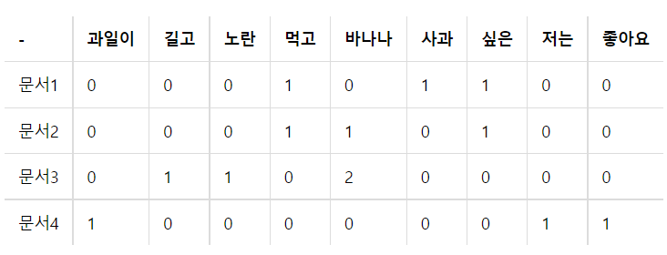
문서1: 저는 사과랑 바나나를 먹어요
문서2: 우리는 귀여운 강아지가 좋아요
문서3: 저의 깜찍하고 귀여운 강아지가 바나나를 먹어요.
이런 문서가 있다고 생각하자. LDA를 수행할 때 토픽이 몇 개일지 가정은 사용자가 해야함. 2개의 토픽을 찾으라 한다면, k=2. k를 몇으로 지정하냐에 따라 원치않는 이상한 결과가 나올 수 있음. 하이퍼 파라미터는 보통 실험에 의해 얻거나, 경험을 통해 얻을 수도 있음. 우선 해보는 게 중요.
문서3개에 대해 전처리 과정을 거치고 DTM을 생성해 LDA의 입력으로 썼다고 가정하자.
<각 문서의 토픽 분포>
문서1: 토픽 A 100%
문서2: 토픽 B 100%
문서3: 토픽 A 40%, B 60%
<각 토픽의 단어 분포>
토픽A: 사과 20%, 바나나 40%, 먹어요 40%, 귀여운 0%, 강아지 0%, 깜찌갛고 0%, 좋아요 0%
토픽B: 사과 0%, 바나나 0%, 먹어요 0%, 귀여운 33%, 강아지 33%, 깜찍하고 16%, 좋아요 16%
이런식으로 분포를 생성해 냄.
LDA는 토픽의 제목을 정해주진 않음. 위 결과로부터 두 토픽이 각각 과일에 대한 토픽과 강아지에 대한 토픽이라 판단해볼 수 있음.
2. LDA 가정
LDA는 빈도수 기반의 표현방식 BoW, DTM, TF-IDF를 입력으로 하는데, 이로부터 알 수 있는 사실은 LDA는 단어의 순서를 신경쓰지 않는다.
- 문서에 사용할 단어의 개수 N을 정한다
- 문서에 사용할 토픽의 혼합을 확률 분포에 기반해 결정
- 위 예제처럼 토픽이 2개면 60%, 40% 이런식으로 설정 가능.
- 문서에 사용할 각 단어를 정한다
3-1) 토픽 분포에서 토픽 T를 확률적으로 고름.- ex) 60%로 강아지를, 40%로 과일 토픽을 선택
3-2) 선택한 토픽 T에서 단어의 출현 확률 분포에 기반해 문서에 사용할 단어 선택 - ex) 강아지를 선택했다면, 33% 확률로 강아지를(토픽B이므로). 3)을 반복하면서 문서를 완성한다.
- ex) 60%로 강아지를, 40%로 과일 토픽을 선택
이런 과정을 통해 문서가 작성됐다는 가정 하에 LDA는 토픽을 뽑기위해 역으로 추적하는 역공학을 수행.
3. LDA 수행하기
1) 알고리즘에게 토픽의 개수 k개를 알려줌.
- k를 입력받으면 k개 토픽이 M개 전체 문서에 걸쳐 분포되어 있다 가정.
2) 모든 단어를 k개 중 하나의 토픽에 할당
- 모든 문서의 단어에 대해 k개 중 하나의 토픽을 랜덤하게 할당. 이게 끝나면 각 문서는 토픽을 갖고, 토픽은 단어 분포를 가지게 된다. 물론, 랜덤 할당이므로 실제로는 틀린 결과. 랜덤 할당이므로 같은 단어라도 다른 토픽에 할당될 수 있음!
3) 모든 문서에 대해 아래를 반복
3-1) 어떤 문서의 각 단어w는 자신은 잘못된 토픽을 할당받았지만, 다른 단어들은 전부 올바르 토픽에 할당되어졌다 가정. 이에 따라 w는 두 가지 기준에 따라 재할당됨.
- p(topic t | document d): 문서 d 단어들 중 토픽 t에 해당하는 단어들의 비율
- p(word w | topic t): 각 토픽들 t에서 해당 단어 w의 분포
이를 반복하다보면, 모든 할당이 수렴이 됨.
4. 잠재 디리클레 할당과 잠재 의미 분석의 차이
LSA : DTM을 차원 축소 하여 축소 차원에서 근접 단어들을 토픽으로 묶는다.
LDA : 단어가 특정 토픽에 존재할 확률과 문서에 특정 토픽이 존재할 확률을 결합확률로 추정하여 토픽을 추출한다.
5. 실습을 통한 이해
LDA는 gensim을 사용. 사이킷런을 통해서도 LDA가 가능.
사이킷런으로 LDA 실습
1) 정수 인코딩과 단어 집합 만들기
앞서 실습한 20개 다른 주제를 가진 뉴스 데이터를 다시 사용. 동일한 전처리를 거친 후에 tokenized_doc으로 저장한 상태.
tokenized_doc[:5]0 [well, sure, story, seem, biased, disagree, st...
1 [yeah, expect, people, read, actually, accept,...
2 [although, realize, principle, strongest, poin...
3 [notwithstanding, legitimate, fuss, proposal, ...
4 [well, change, scoring, playoff, pool, unfortu...
Name: clean_doc, dtype: object각 단어에 정수 인코딩을 하며, 뉴스에서의 빈도를 기록.
각 단어를 (word_id, word_frequency)의 형태로 바꿈. word_id가 인코딩된 값, freq는 뉴스에서 해당 단어의 빈도수를 의미.
from gensim import corpora
dictionary = corpora.Dictionary(tokenized_doc)
corpus = [dictionary.doc2bow(text) for text in tokenized_doc]
print(corpus[1]) # 수행된 결과에서 두 번째 뉴스. 첫 뉴스의 인덱스는 0
[(52, 1), (55, 1), (56, 1), (57, 1), (58, 1), (59, 1), (60, 1), (61, 1), (62, 1), (63, 1), (64, 1), (65, 1), (66, 2), (67, 1), (68, 1), (69, 1), (70, 1), (71, 2), (72, 1), (73, 1), (74, 1), (75, 1), (76, 1), (77, 1), (78, 2), (79, 1), (80, 1), (81, 1), (82, 1), (83, 1), (84, 1), (85, 2), (86, 1), (87, 1), (88, 1), (89, 1)](52, 1)은 52라는 단어가 두 번째 뉴스에서 1번 등장했음을 알려준다. 이게 뭘까?
print(dictionary[52])wellwell임을 알 수 있음. 단어의 학습된 개수를 확인해보자
len(dictionary)64281총 64,281개의 단어가 학습됨. LDA를 훈련해보자.
2) LDA 훈련
import gensim
t = 20 # 20개의 토픽
ldamodel = gensim.models.ldamodel.LdaModel(corpus, num_topics = t, id2word = dictionary, passes = 15)
## 기여도 상위 4개 단어만 할당
topics = ldamodel.print_topics(num_words = 4)
for topic in topics:
    print(topic)
lda는 corpus, topics, index등을 인자로 가짐
(0, '0.008*"people" + 0.008*"jesus" + 0.008*"would" + 0.006*"believe"')
(1, '0.019*"file" + 0.012*"program" + 0.009*"files" + 0.008*"available"')
(2, '0.019*"would" + 0.012*"like" + 0.011*"know" + 0.011*"people"')
(3, '0.006*"professor" + 0.005*"ancient" + 0.004*"university" + 0.004*"reuss"')
(4, '0.020*"encryption" + 0.019*"chip" + 0.015*"clipper" + 0.014*"keys"')
(5, '0.016*"entries" + 0.012*"contest" + 0.006*"winners" + 0.005*"borland"')
(6, '0.019*"space" + 0.007*"nasa" + 0.004*"launch" + 0.004*"data"')
(7, '0.016*"government" + 0.008*"american" + 0.006*"rights" + 0.006*"states"')
(8, '0.009*"bike" + 0.008*"good" + 0.007*"thanks" + 0.006*"used"')
(9, '0.012*"drive" + 0.010*"card" + 0.009*"windows" + 0.009*"system"')
(10, '0.010*"nrhj" + 0.007*"wwiz" + 0.006*"bxom" + 0.006*"gizw"')
(11, '0.013*"remark" + 0.012*"simms" + 0.008*"auto" + 0.006*"autos"')
(12, '0.010*"period" + 0.008*"play" + 0.007*"team" + 0.007*"season"')
(13, '0.014*"said" + 0.009*"went" + 0.007*"home" + 0.007*"people"')
(14, '0.010*"university" + 0.008*"national" + 0.008*"april" + 0.007*"information"')
(15, '0.012*"israel" + 0.011*"jews" + 0.011*"armenian" + 0.010*"turkish"')
(16, '0.006*"control" + 0.005*"guns" + 0.005*"crime" + 0.004*"system"')
(17, '0.008*"pain" + 0.008*"list" + 0.007*"medical" + 0.007*"please"')
(18, '0.018*"game" + 0.012*"team" + 0.011*"year" + 0.011*"good"')
(19, '0.009*"mail" + 0.007*"internet" + 0.006*"used" + 0.006*"system"')
각 단어 앞에 붙은 수치는 해당 토픽에 대한 기여도를 보여줌.
각 토픽에 어떤 단어들이 할당되었는지 보면 된다. passes는 알고리즘의 동작 횟수(수렴을 위한 반복의 횟수) 이것도 hyper-param..
print_topics()의 default는 10!
3) LDA 시각화 하기
pyLDAvis 설치가 필요.
pip install pyLDAvis코랩에서 설치했다면, 설치 후 런타임 재시작 필요!
import pyLDAvis.gensim
pyLDAvis.enable_notebook()
vis = pyLDAvis.gensim.prepare(ldamodel, corpus, dictionary)
pyLDAvis.display(vis)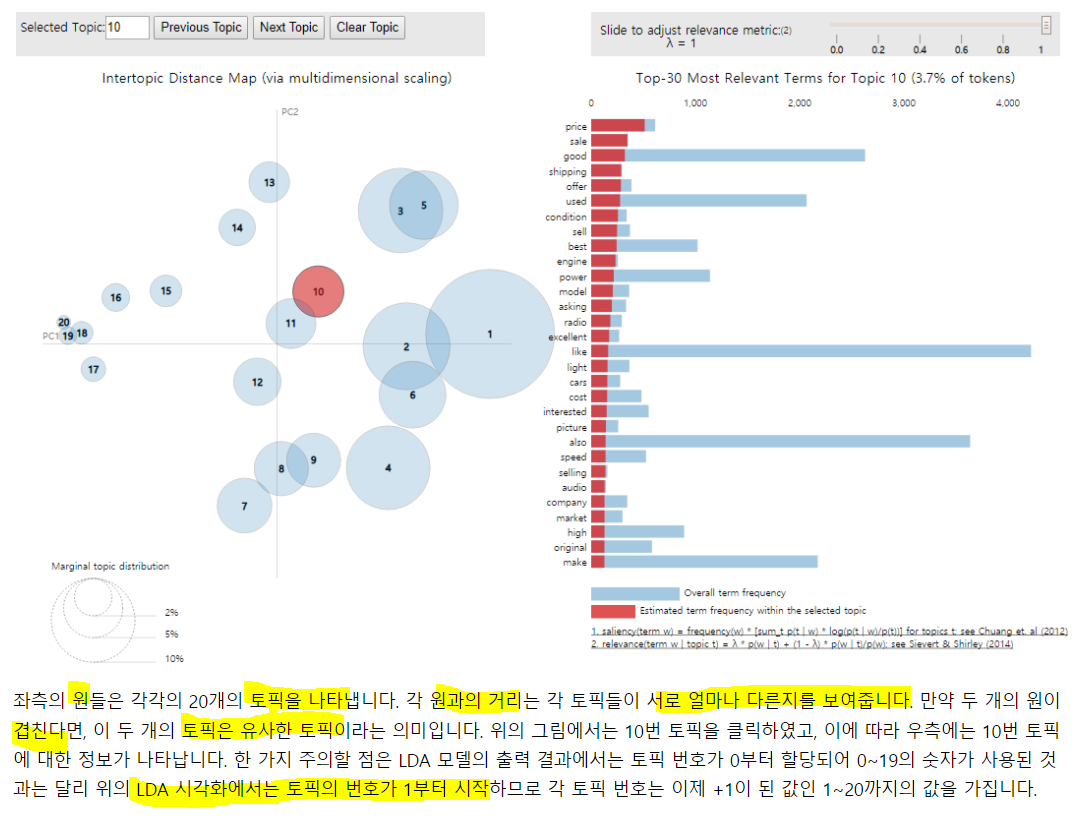
4) 문서 별 토픽 분포 보기
토픽 별 단어 분포는 봤지만, 문서 별 토픽 분포는 확인 못했음. ldamodel[]에 전체 데이터가 정수 인코딩 된 결과를 넣으면 확인 가능.
상위 5개 문서에 대해서만 토픽 분포를 확인
for i, topic_list in enumerate(ldamodel[corpus]):
    if i == 5:
        break
    print(i, '번째 문서의 topic 비율은', topic_list)
0 번째 문서의 topic 비율은 [(1, 0.40645686), (14, 0.32995152), (16, 0.24988192)]
1 번째 문서의 topic 비율은 [(14, 0.26643324), (16, 0.6087502), (17, 0.061824974), (18, 0.04347932)]
2 번째 문서의 topic 비율은 [(1, 0.29319322), (2, 0.12145591), (6, 0.14717588), (11, 0.047261782), (14, 0.13408786), (16, 0.245535)]
3 번째 문서의 topic 비율은 [(1, 0.4929492), (3, 0.31348726), (12, 0.032681946), (16, 0.1489413)]
4 번째 문서의 topic 비율은 [(8, 0.32045797), (9, 0.12288789), (17, 0.5251727)]숫자는 토픽의 번호를, 확률은 해당 문서에서 차지하는 비율을 의미. 0 번째 문서에서 토픽1이 40%를 차지하는 것.
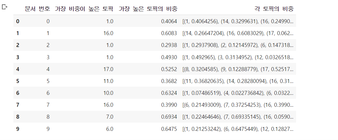
좀 더 깔끔하게 데이터 프레임으로 표현하기
def make_topictable(ldamodel, corpus):
    topic_table = pd.DataFrame()

    # 문서의 번호와 문서의 토픽 비중을 한 줄씩 꺼내옴
    for i, topic_list in enumerate(ldamodel[corpus]):
        ## ldamodel.per_word_topics가 True면 topic_list[0]을 fasle면 topic_list 전체를 할당
        doc = topic_list[0] if ldamodel.per_word_topics else topic_list
        doc = sorted(doc, key = lambda x: (x[1]), reverse = True)
        ## 각 문서에 대해 비중이 높은 토픽순으로 정렬

        for j, (topic_num, prop_topic) in enumerate(doc): # 몇 번 토픽인지와 비중을 나눠서 저장
            if j == 0:
                ## 정렬을 한 상태이므로 가장 앞이 비중이 높음
                topic_table = topic_table.append(pd.Series([int(topic_num), round(prop_topic, 4), topic_list]), ignore_index = True)
            else:
                break
    return (topic_table)
topictable = make_topictable(ldamodel, corpus)
topictable = topictable.reset_index() # 문서 번호를 의미하는 열로 사용하기 위해 인덱스를 추가
topictable.columns = ['문서 번호', '가장 비중이 높은 토픽', '가장 높은 토픽의 비중', '각 토픽의 비중']
topictable[:10]LDA는 지도학습이므로, 토픽을 알고 있고 이에 따라 분류하는 것. 0~19에 대한 정보가 없어서 어떤 토픽을 의미하는 진 모르겠음
dataset.target_names을 보면 각 토픽이 뭔지 알 수 있음. 어떻게 보면 비지도 학습이 될 수 있을듯. 그룹화 가능하므로. LDA를 활용해 문서 별 그룹화 -> clustering이 되는 것이라 생각.
비중이 높은 토픽으로 해당 문서의 주제를 나눌듯?
참고 링크
http://s-space.snu.ac.kr/bitstream/10371/95582/1/22_1_%EB%82%A8%EC%B6%98%ED%98%B8.pdf
https://bab2min.tistory.com/568
https://annalyzin.wordpress.com/2015/06/21/laymans-explanation-of-topic-modeling-with-lda-2/
https://towardsdatascience.com/latent-dirichlet-allocation-15800c852699
https://radimrehurek.com/gensim/wiki.html#latent-dirichlet-allocation
https://www.machinelearningplus.com/nlp/topic-modeling-gensim-python/
모델 저장 및 로드 하기 : https://stackabuse.com/python-for-nlp-working-with-the-gensim-library-part-2/
전반적으로 참고하기 좋은 글 : https://shichaoji.com/2017/04/25/topicmodeling/
동영상 강의 : https://blog.naver.com/chunjein/220946362463
뉴스를 가지고 할 수 있는 다양한 일들 : https://www.slideshare.net/koorukuroo/20160813-pycon2016apac
3) LDA 실습2
2번에선 gensim을 이용해 LDA를 했고, 이번엔 사이킷런을 이용
전반적 과정은 LSA와 유사
1. 실습을 통한 이해
1) 뉴스 기사 제목 데이터에 대한 이해
약 15년간 발행된 뉴스 기사 제목을 모아놓은 영어 데이터를 다운로드
다운로드
import pandas as pd
import urllib.request
urllib.request.urlretrieve("https://raw.githubusercontent.com/franciscadias/data/master/abcnews-date-text.csv", filename="abcnews-date-text.csv")
data = pd.read_csv('abcnews-date-text.csv', error_bad_lines=False)
링크에서 안받고, urllib를 이용해서 github에서 다운받을 수 있음
저 url을 read_csv에 넣어도 읽어오긴 함.
print(len(data))1082168108만개의 샘플을 갖고 있음.
data.head()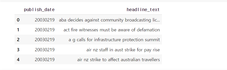
data는 날짜와 헤드라인으로 구성.
## [[ ]]로 원래는 시리즈 형태를 데이터 프레임의 형태로 불러옴
text = data[['headline_text']]
text.head()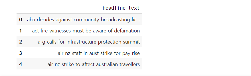
2) 텍스트 전처리
불용어 제거, 표제어 추출(stemming), 길이가 짧은 단어 제거!!
import nltk
nltk.download('punkt')
text['headline_text'] = text.apply(lambda x: nltk.word_tokenize(x['headline_text']), axis = 1)
print(text.head())
NLTK의 tokenize를 이용해 100만개의 텍스트를 tokenizing! 상위 5개만 확인
                                       headline_text
0  [aba, decides, against, community, broadcastin...
1  [act, fire, witnesses, must, be, aware, of, de...
2  [a, g, calls, for, infrastructure, protection,...
3  [air, nz, staff, in, aust, strike, for, pay, r...
4  [air, nz, strike, to, affect, australian, trav...
NLTK가 제공하는 영어 불용어 통해 text를 제거
from nltk.corpus import stopwords
stop = stopwords.words('english')
text['headline_text'] = text['headline_text'].apply(lambda x: [word for word in x if word not in (stop)])
## 불용어 삭제되고 상위 5개 text
print(text.head())
headline_text
0 [aba, decides, community, broadcasting, licence]
1 [act, fire, witnesses, must, aware, defamation]
2 [g, calls, infrastructure, protection, summit]
3 [air, nz, staff, aust, strike, pay, rise]
4 [air, nz, strike, affect, australian, travellers]- 확실히 제거하지 전과 후만 비교해도 차이가 보임!
표제어 추출을 수행. 3인칭 단수 표현을 1인칭으로 바꾸고, 과거 현재형 동사를 현재형으로 바꿈!
nltk.download('wordnet')
from nltk.stem import WordNetLemmatizer
text['headline_text'] = text['headline_text'].apply(lambda x: [WordNetLemmatizer().lemmatize(word, pos = 'v') for word in x])
print(text.head())
headline_text
0 [aba, decide, community, broadcast, licence]
1 [act, fire, witness, must, aware, defamation]
2 [g, call, infrastructure, protection, summit]
3 [air, nz, staff, aust, strike, pay, rise]
4 [air, nz, strike, affect, australian, travellers]표제어 추출이 완료됐고, 길이가 3이하인 단어 제거
tokenized_doc = text['headline_text'].apply(lambda x: [word for word in x if len(word) > 3])
print(tokenized_doc[:5])
0 [decide, community, broadcast, licence]
1 [fire, witness, must, aware, defamation]
2 [call, infrastructure, protection, summit]
3 [staff, aust, strike, rise]
4 [strike, affect, australian, travellers]3) TF-IDF 행렬 만들기
사이킷런의 TfidfVectorize는 텍스트 자체를 입력으로 받으므로 역토큰화 필요
detokenized_doc = []
for i in range(len(text)):
    t = ' '.join(tokenized_doc[i])
    detokenized_doc.append(t)

text['headline_text'] = detokenized_doc
text.head()
토큰의 수를 1000개로 제한해 TF-IDF 생성
from sklearn.feature_extraction.text import TfidfVectorizer
vectorizer = TfidfVectorizer(stop_words = 'english', max_features = 1000)
X = vectorizer.fit_transform(text['headline_text'])
X.shape
(1082168, 1000)1000개의 단어를 가지고 108만개의 doc에 대한 TF-IDF 생성
4) 토픽 모델링
from sklearn.decomposition import LatentDirichletAllocation
lda_model = LatentDirichletAllocation(n_components = 10, learning_method = 'online', random_state = 777, max_iter = 1)
lda_top = lda_model.fit_transform(X)
print(lda_model.components_)
print(lda_model.components_.shape)
[[1.00001533e-01 1.00001269e-01 1.00004179e-01 ... 1.00006124e-01
1.00003111e-01 1.00003064e-01]
[1.00001199e-01 1.13513398e+03 3.50170830e+03 ... 1.00009349e-01
1.00001896e-01 1.00002937e-01]
[1.00001811e-01 1.00001151e-01 1.00003566e-01 ... 1.00002693e-01
1.00002061e-01 7.53381835e+02]
...
[1.00001065e-01 1.00001689e-01 1.00003278e-01 ... 1.00006721e-01
1.00004902e-01 1.00004759e-01]
[1.00002401e-01 1.00000732e-01 1.00002989e-01 ... 1.00003517e-01
1.00001428e-01 1.00005266e-01]
[1.00003427e-01 1.00002313e-01 1.00007340e-01 ... 1.00003732e-01
1.00001207e-01 1.00005153e-01]]
(10, 1000)terms = vectorizer.get_feature_names()
def get_topics(components, feature_names, n = 5):
for idx, topic in enumerate(components):
print('Topic: {}'.format(idx + 1), [(feature_names[i], topic[i].round(2)) for i in topic.argsort()[: -n-1: -1]])
get_topics(lda_model.components_, terms)Topic: 1 [('government', 8725.19), ('sydney', 8393.29), ('queensland', 7720.12), ('change', 5874.27), ('home', 5674.38)]
Topic: 2 [('australia', 13691.08), ('australian', 11088.95), ('melbourne', 7528.43), ('world', 6707.7), ('south', 6677.03)]
Topic: 3 [('death', 5935.06), ('interview', 5924.98), ('kill', 5851.6), ('jail', 4632.85), ('life', 4275.27)]
Topic: 4 [('house', 6113.49), ('2016', 5488.19), ('state', 4923.41), ('brisbane', 4857.21), ('tasmania', 4610.97)]
Topic: 5 [('court', 7542.74), ('attack', 6959.64), ('open', 5663.0), ('face', 5193.63), ('warn', 5115.01)]
Topic: 6 [('market', 5545.86), ('rural', 5502.89), ('plan', 4828.71), ('indigenous', 4223.4), ('power', 3968.26)]
Topic: 7 [('charge', 8428.8), ('election', 7561.63), ('adelaide', 6758.36), ('make', 5658.99), ('test', 5062.69)]
Topic: 8 [('police', 12092.44), ('crash', 5281.14), ('drug', 4290.87), ('beat', 3257.58), ('rise', 2934.92)]
Topic: 9 [('fund', 4693.03), ('labor', 4047.69), ('national', 4038.68), ('council', 4006.62), ('claim', 3604.75)]
Topic: 10 [('trump', 11966.41), ('perth', 6456.53), ('report', 5611.33), ('school', 5465.06), ('woman', 5456.76)]