
Two versions of the problem
- 0-1 knapsack problem
- Items are indivisible: you either take an item or not ➡️ DP (Greedy X)
- Fractional knapsack problem
- Items are divisible: you can take any fraction of an item ➡️ Greedy
- compute the value per pound vi/wi for each item
- For greedy strategy, the thief begins by taking as much as possible of the item with the greatest value per pound, continue
➡️ Both problem optrmal substructure property, but ony fractronal greedy choice property
0-1 knapsack problem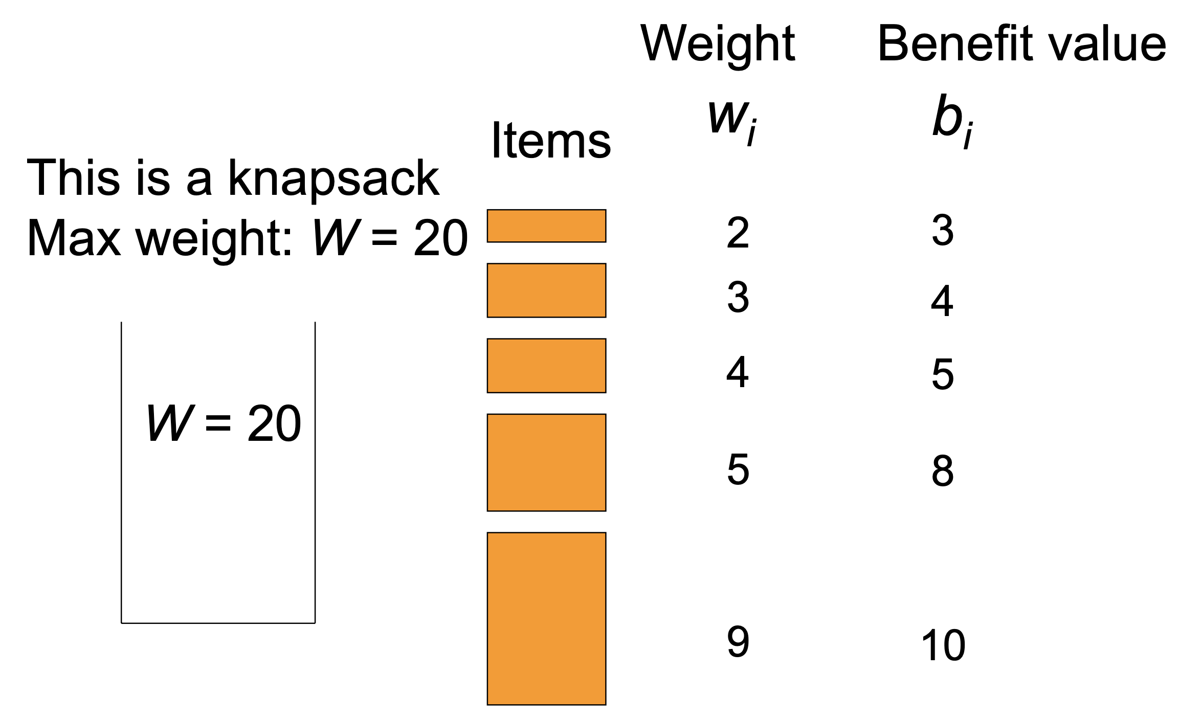
[1] Brute force approach
- Since there are n items, there are possible combinations of items
- We go through(살펴보다) all combinations and find the one with the most total value and with total weight less or equal to W
- Running time will be Θ()
[2] Greedy
: does not work for this problem
[3] Dynamic programming
- identifying the subproblems is important
- If items are labeled 1..n, S = { items labeled 1, 2, .. k } ➡️ 가장 간단한 방법
- This is a valid subproblem definition- Q. Can we describe the final solution (S) in terms of subproblems (S)?
- A. Unfortunately, we can't do that
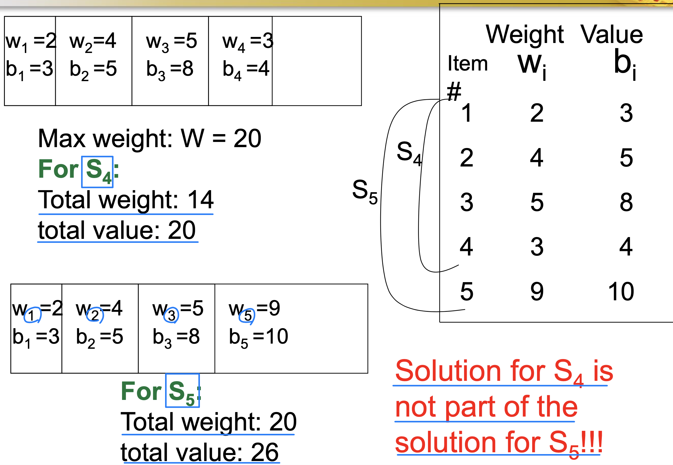
- So current definition of a subproblem is flawed(결함이 있다) and we need another one!
- Add another parameter: w, which will represent the exact weight for each subset of items
- The subproblem then will be B[k,w]
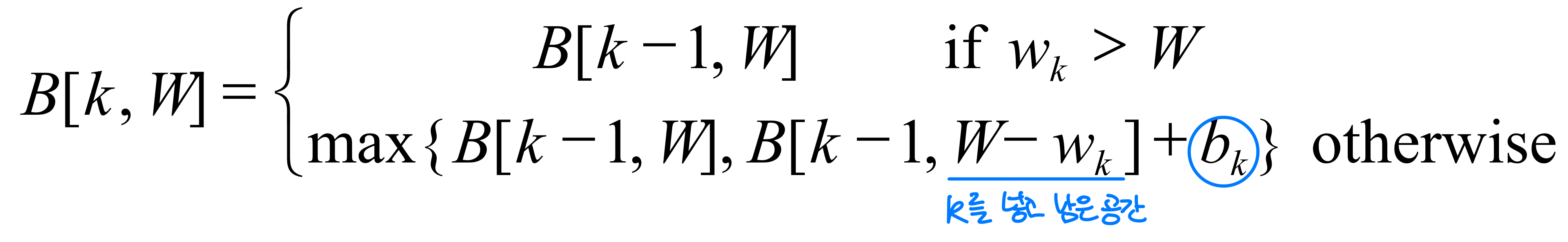
- The best subset of S that has the total weight W, either contains item k or not (k를 넣을지 말지)
- First case: w > W. Item k can’t be part of the solution
- Second case: w <= W. Item k may be in the solution, and we choose the case with greater value
for w = 0 to W
B[0, w] = 0 // item # = 0
for i = 1 to n
B[i, 0] = 0 // weight = 0
for w = 1 to W
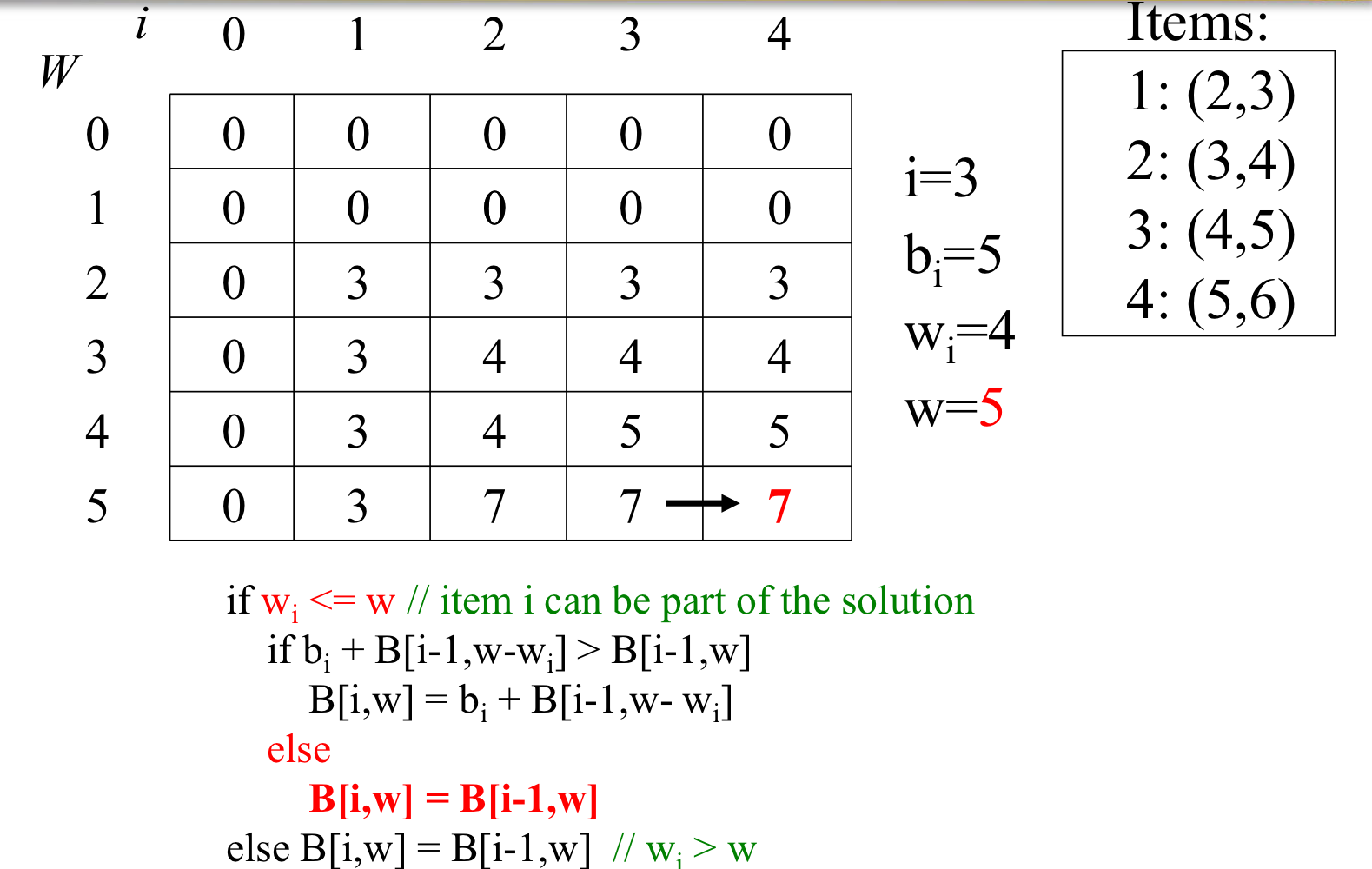
if w[i] <= W // item i can be part of the solution
if b[i] + B[i -1 , W - w[i]] > B[i - 1, W]
B[i, w] = b[i] + B[i - 1, W - w[i]]
else B[i, w] = B[i-1, w]
else B[i, W] = B[i - 1, W] // W[i] > W⭐️ O(nW)
[4] Branch and Bound - Best First Search
-
We do not visit every node, but determine if it is worth(값어치 있는) or not
-
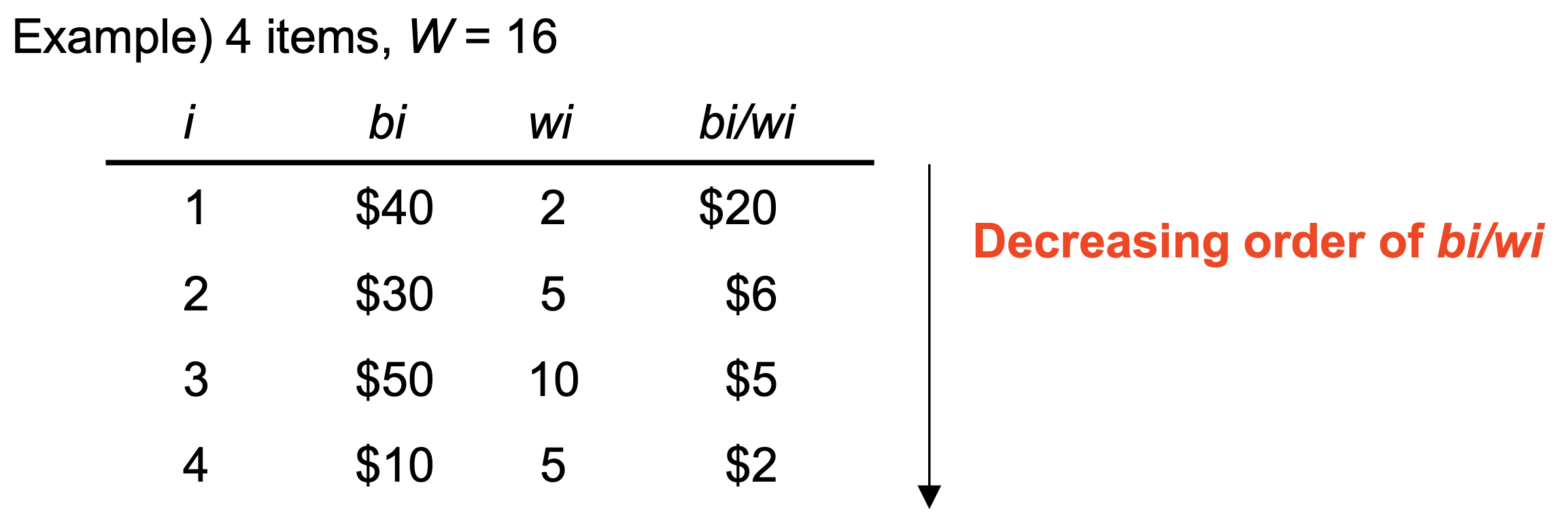
전제 조건 : Sorting in descending order according to b / w (benefit per weight)
-
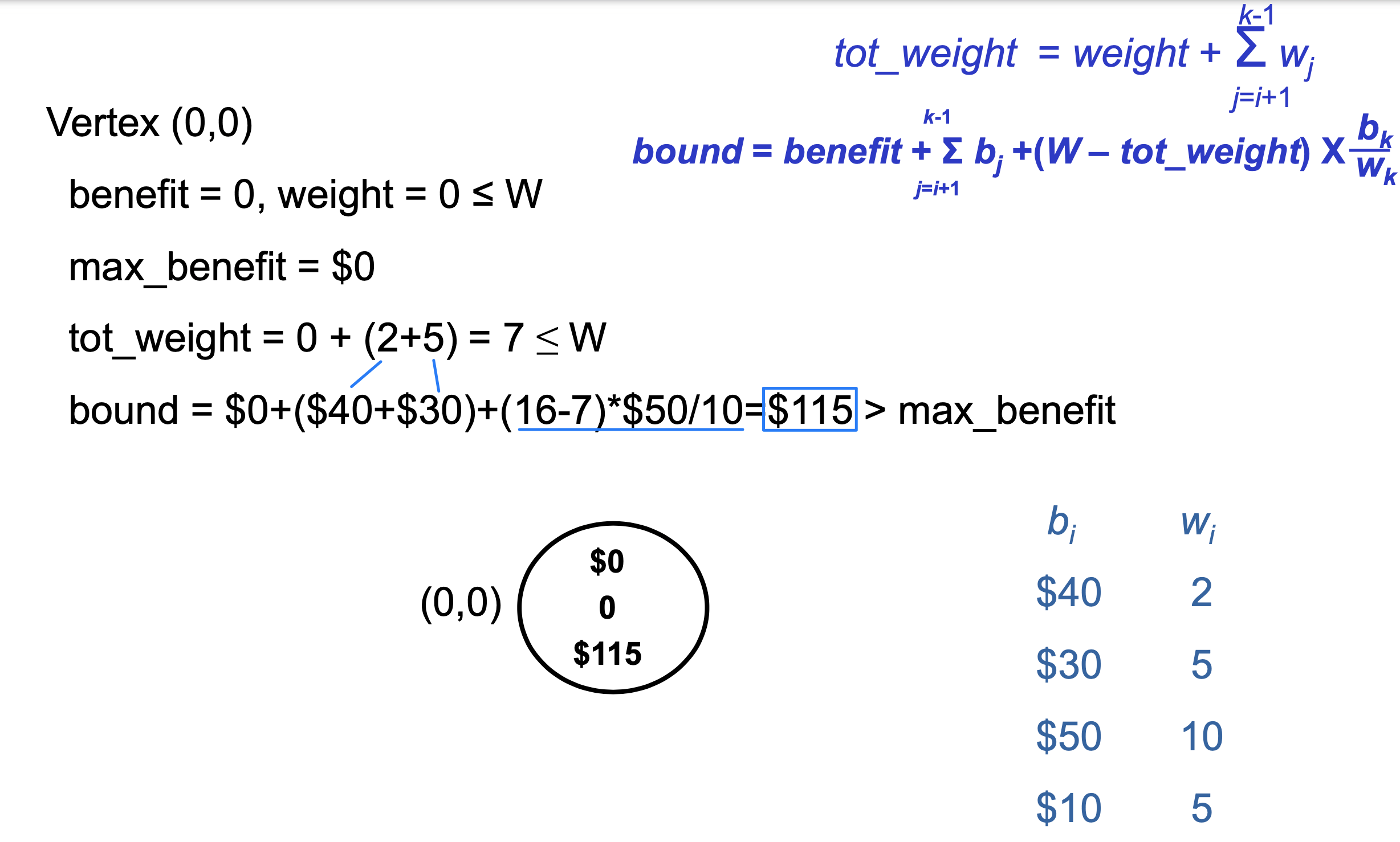
At each node we compute three local values
- benefit : sum of benefit value up to this node
- weight : sum of weights up to this node
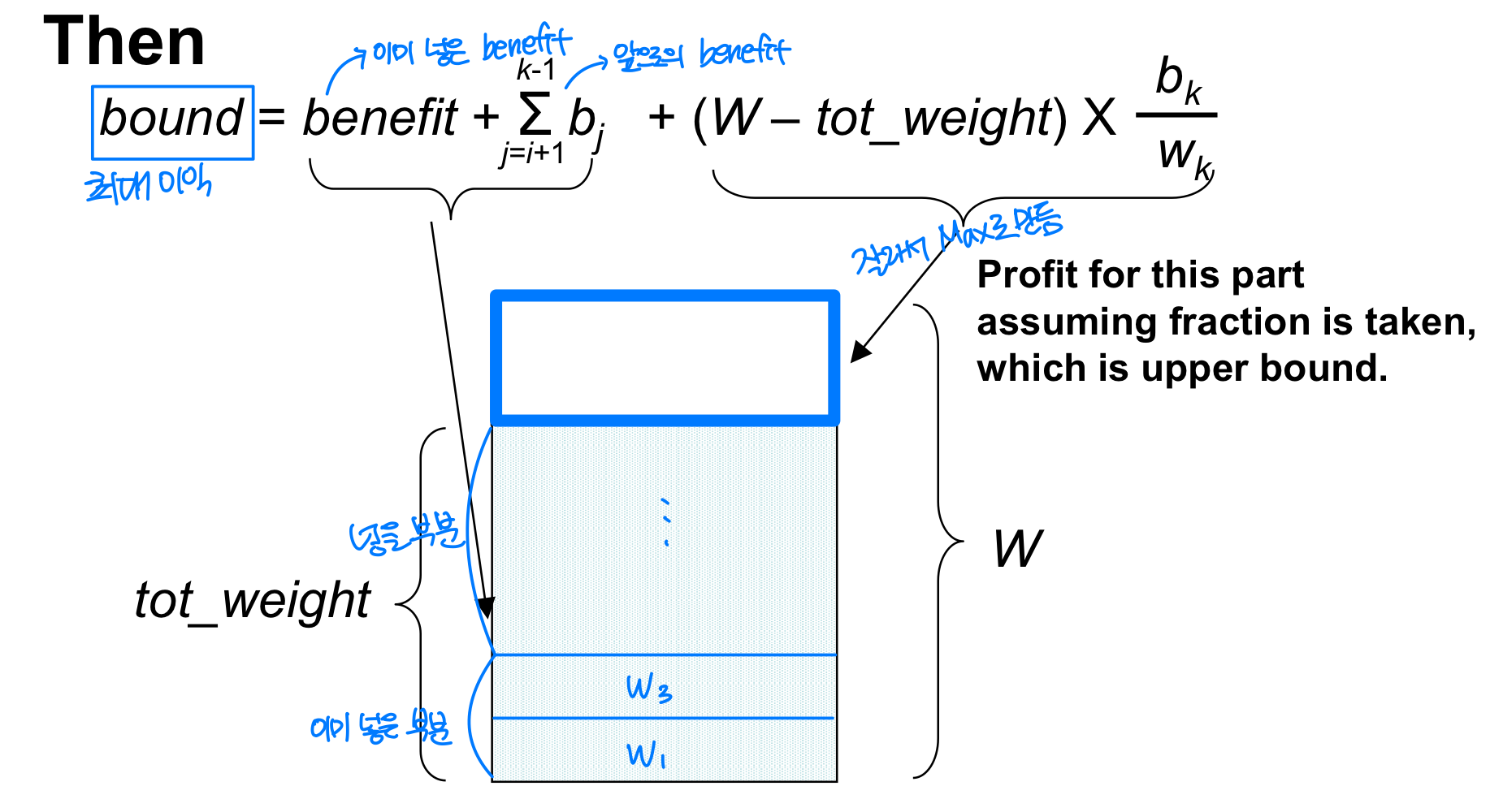
- bound : upper bound on the benefit we could achieve by expanding beyond this node (predict, foresee, forecast)
-
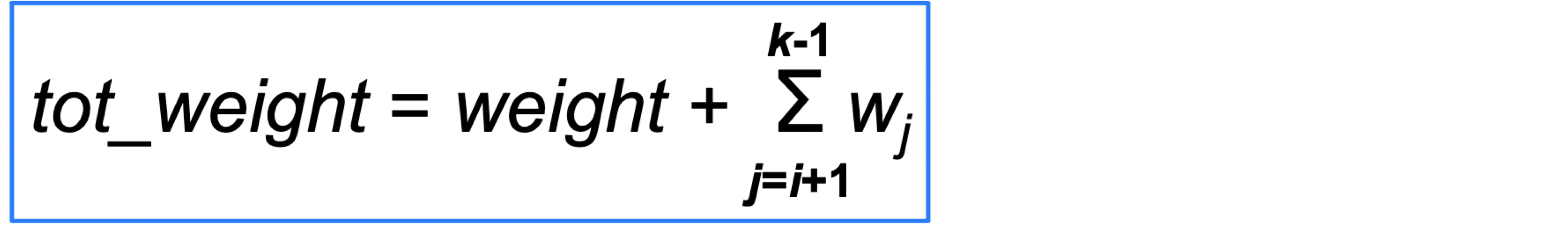
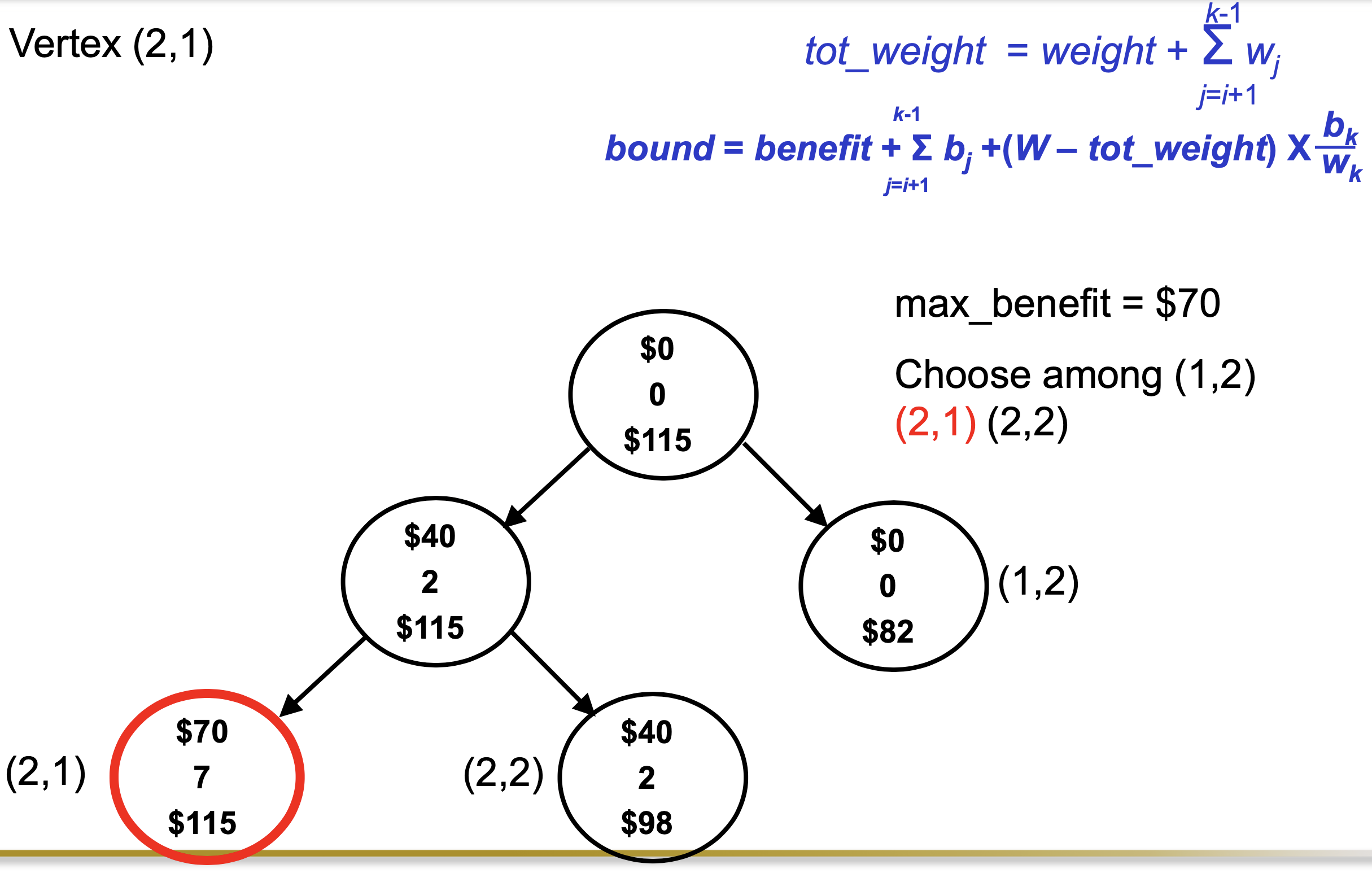
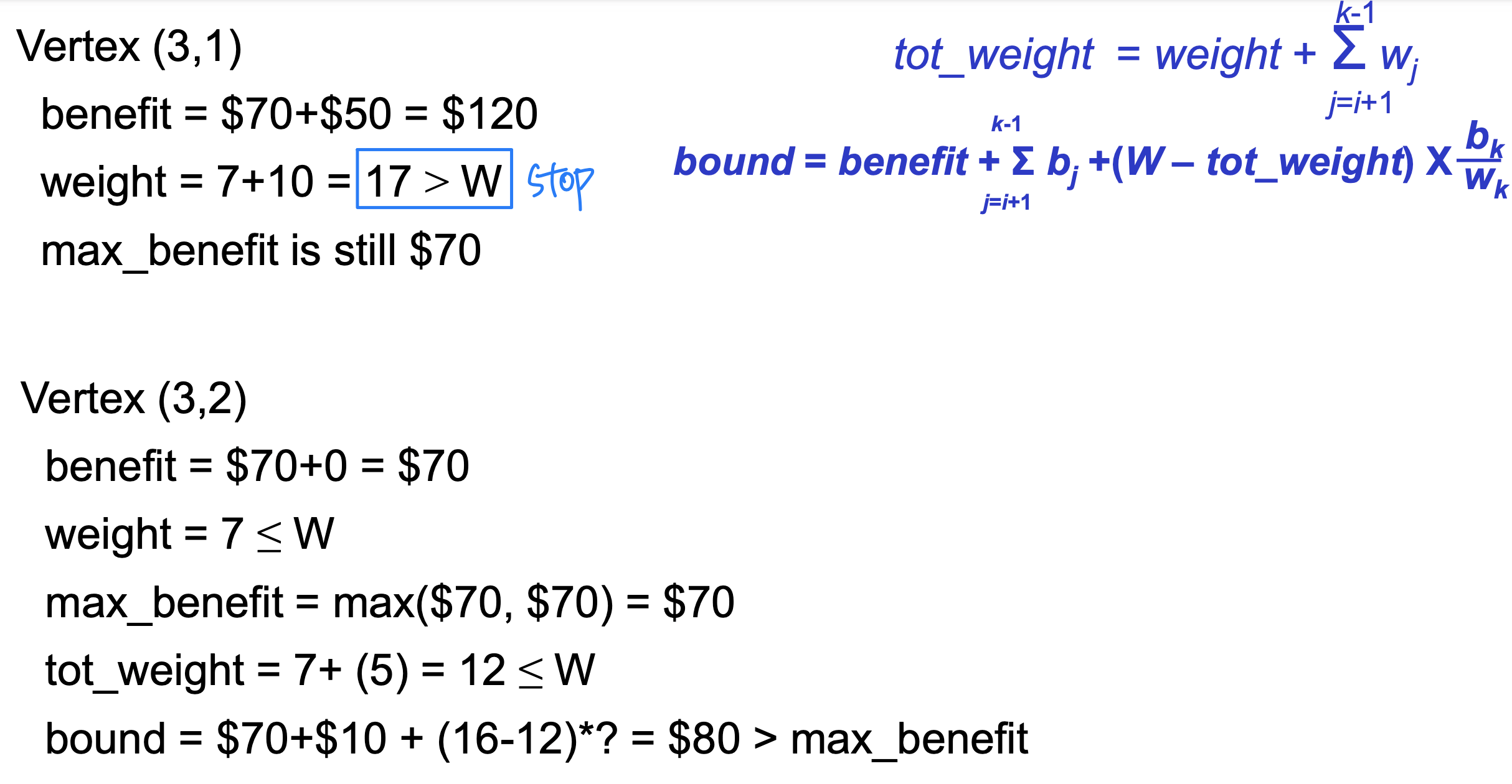
Computing bound
- tot_weight = weight(이미 knapsack에 넣은 총 weight) + 미래에 넣을 weight ( tot_weight <= W )
-
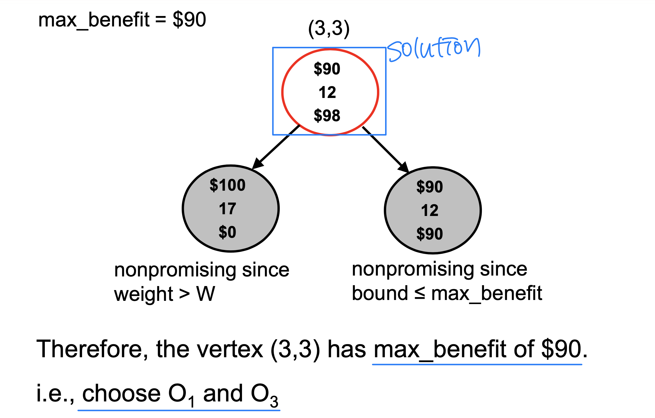
And we need one more global variable max_benefit
: benefit in the best solution found so far- Initially, max_benefit = 0
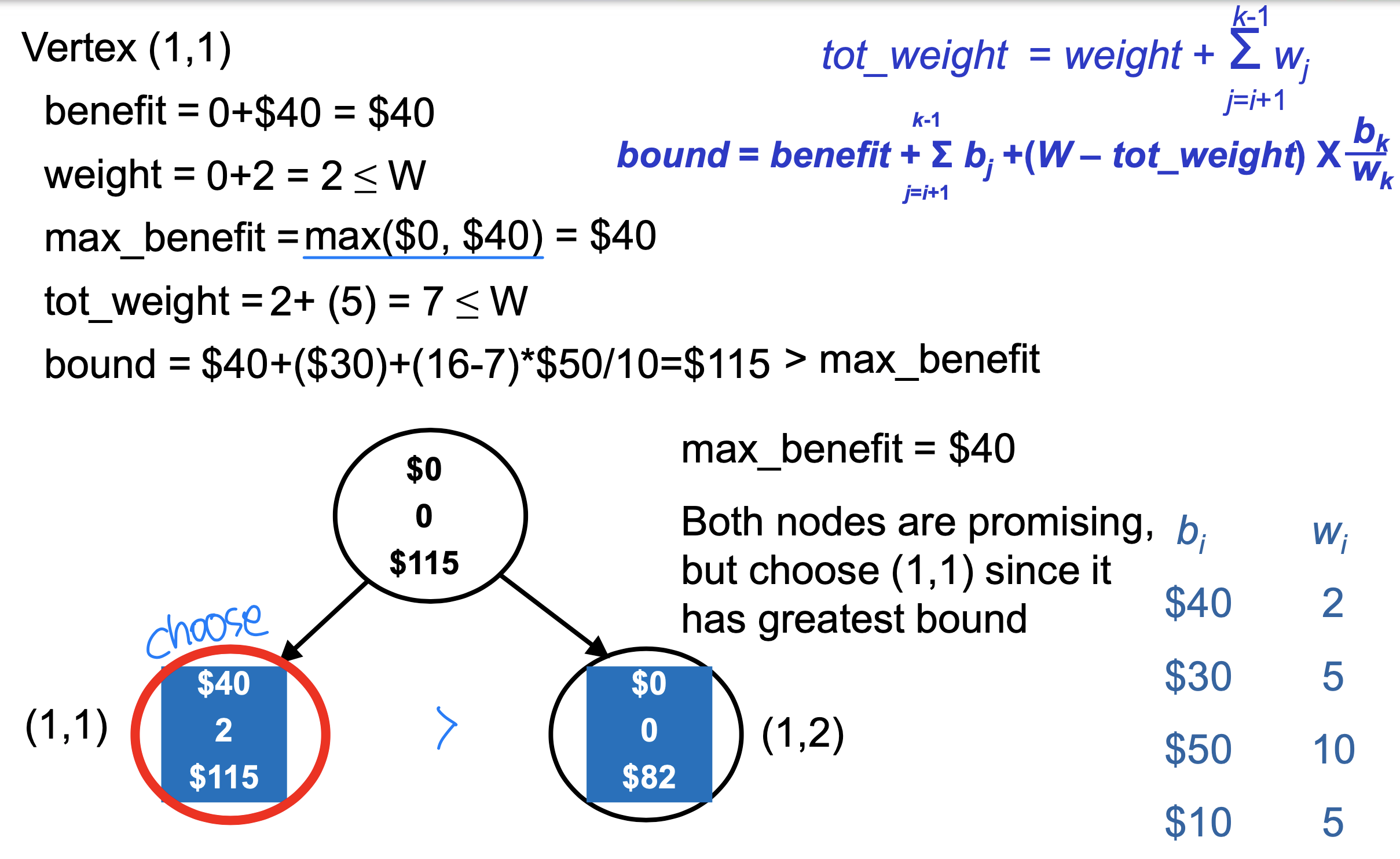
- if weight < W, max_benefit = max(max_benefit, benefit)
- Q. Relationship between local variable ‘bound’ and global variable ‘max_beneit’?
- promising : expand beyond this node
- nonpromising : stop here
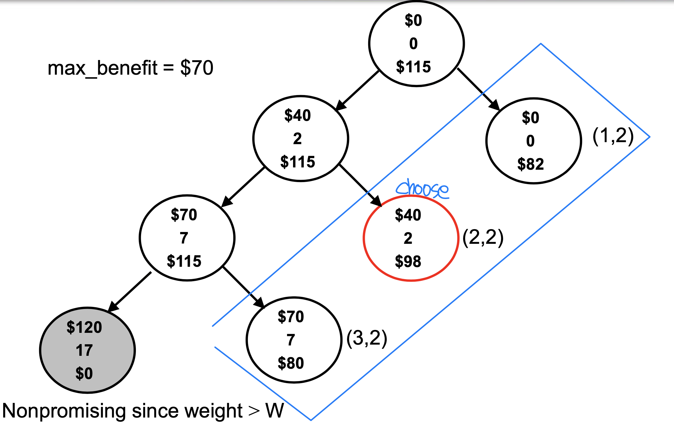
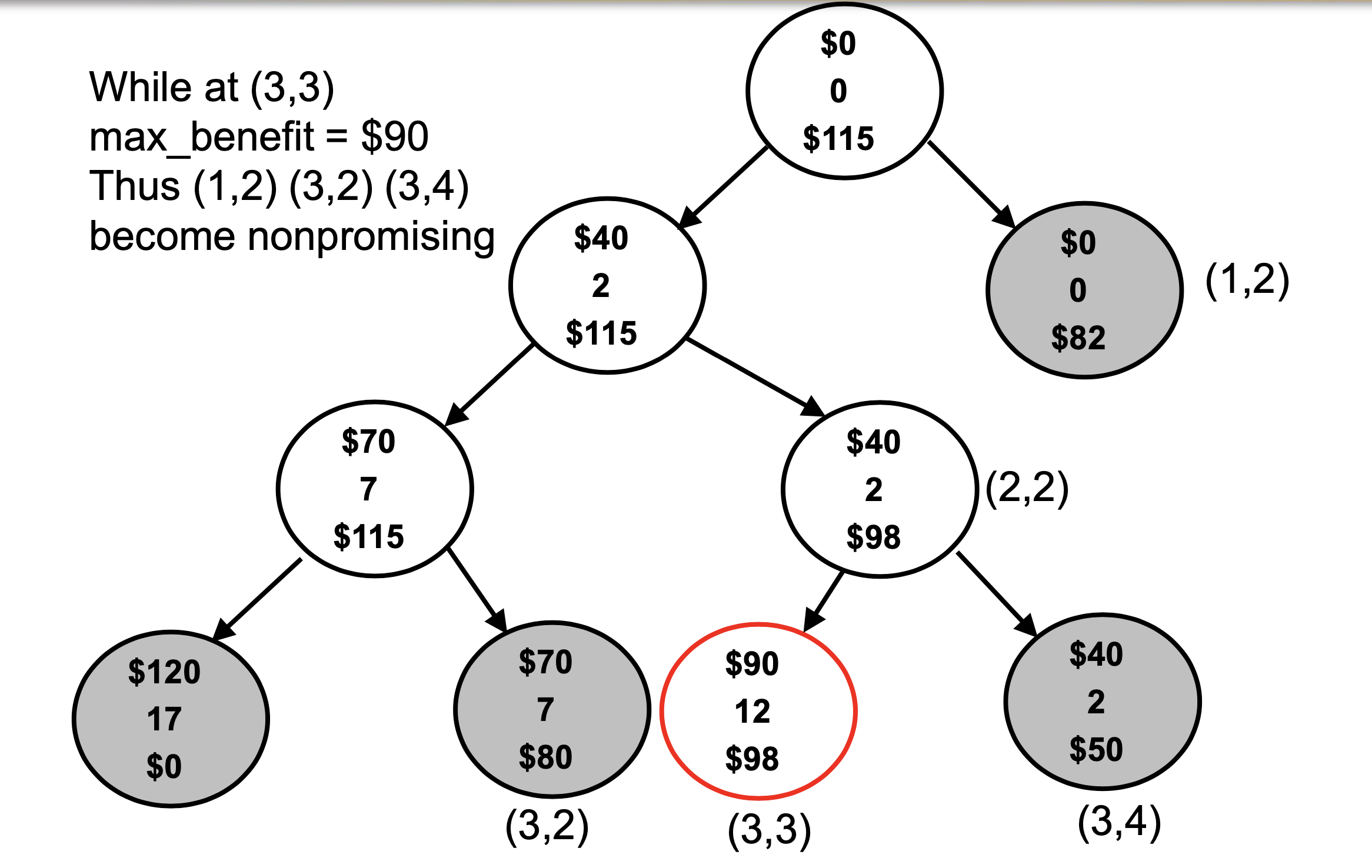
- if bound ≤ max_benefit or weight > W ➡️ nonpromising
- if bound > max_benefit and weight ≤ W ➡️ promising
-
Two non-promising case
- Case 1: bound ≤ max_benefit
- The ‘benefit’ computed at this node is effective
- We just do not expand beyond this node (필요가 없다) - Case 2: weight > W
- The ‘benefit’ computed at this node is not effective
- So ‘max_benefit’ will not be updated and we do not expand beyond this node
- Case 1: bound ≤ max_benefit
-
Basically apply BFS and choose promising(유망한) and unexpanded node with greatest bound
-
Ex_
Exercise in class
1. Knapsack Greedy
Find running time
➡️ (n lg n) : sorting(n lg n) + 1부터 n-1까지 스캔(n)
➕ merge, heap sort만 (n lg n)
2. Knapsack DP
n = 4
W = 4
Elements(w, b) : (2, 3), (3, 4), (4, 5), (5, 6)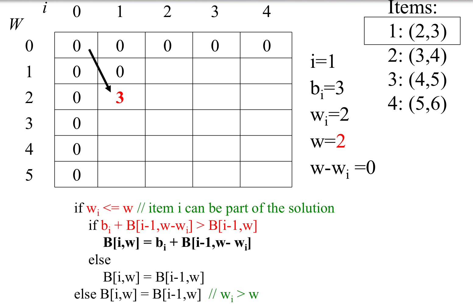
 ➕ DP는 sorting 필요x, Greedy는 필요!
3. Knapsack BB
Total_weight = 10
| i | b | w | b / w |
|---|---|---|---|
| 1 | 30 | 2 | 15 |
| 2 | 60 | 5 | 12 |
| 3 | 70 | 7 | 10 |
| 4 | 20 | 4 | 5 |
➡️ sorted with b / w DES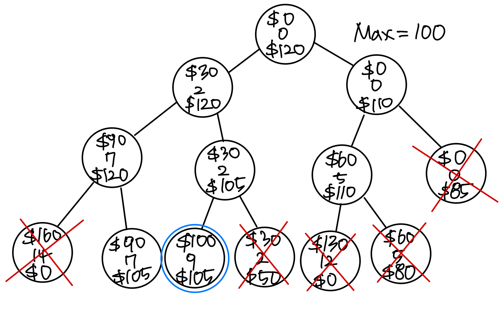
HGU 전산전자공학부 용환기 교수님의 23-1 알고리듬 분석 수업을 듣고 작성한 포스트이며, 첨부한 모든 사진은 교수님 수업 PPT의 사진 원본에 필기를 한 수정본입니다.