
🖥️ Background
Weighted
not weighted
Directed graph (Digraph) : head -> tail
Undirected graphs: Normally an edge can’t connect a vertex to itself
➡️ A graph may not have multiple occurrences of the same edge
Symmetric digraph : For every edge vw, there is also the reverse edge wv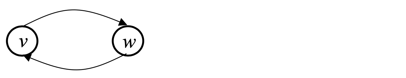 Complete graphs (undirected) : There is an edge with each pair of vertices
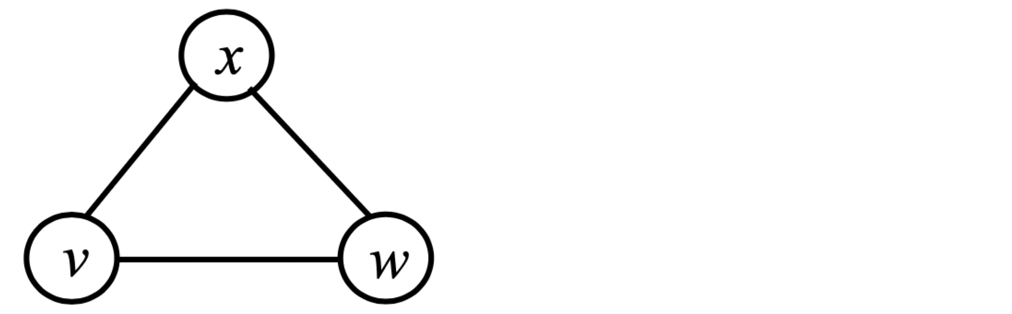 Size of graph
- Number of nodes. Usually n
- Number of edges: Usually m
Dense graph: many edges
- Undirected: Each node connects to all others, so the graph with
m = n(n-1)/2 is called a complete graph
- Directed: m = n(n-1)
Sparse graph: fewer edges ➡️ Could be zero edges...
Path : a sequence of vertices P = (v, v, ..., v) such that, for 1 ≤ i ≤ k, edge (v, v) ∈ E
Path P is simple if no vertex appears more than once in P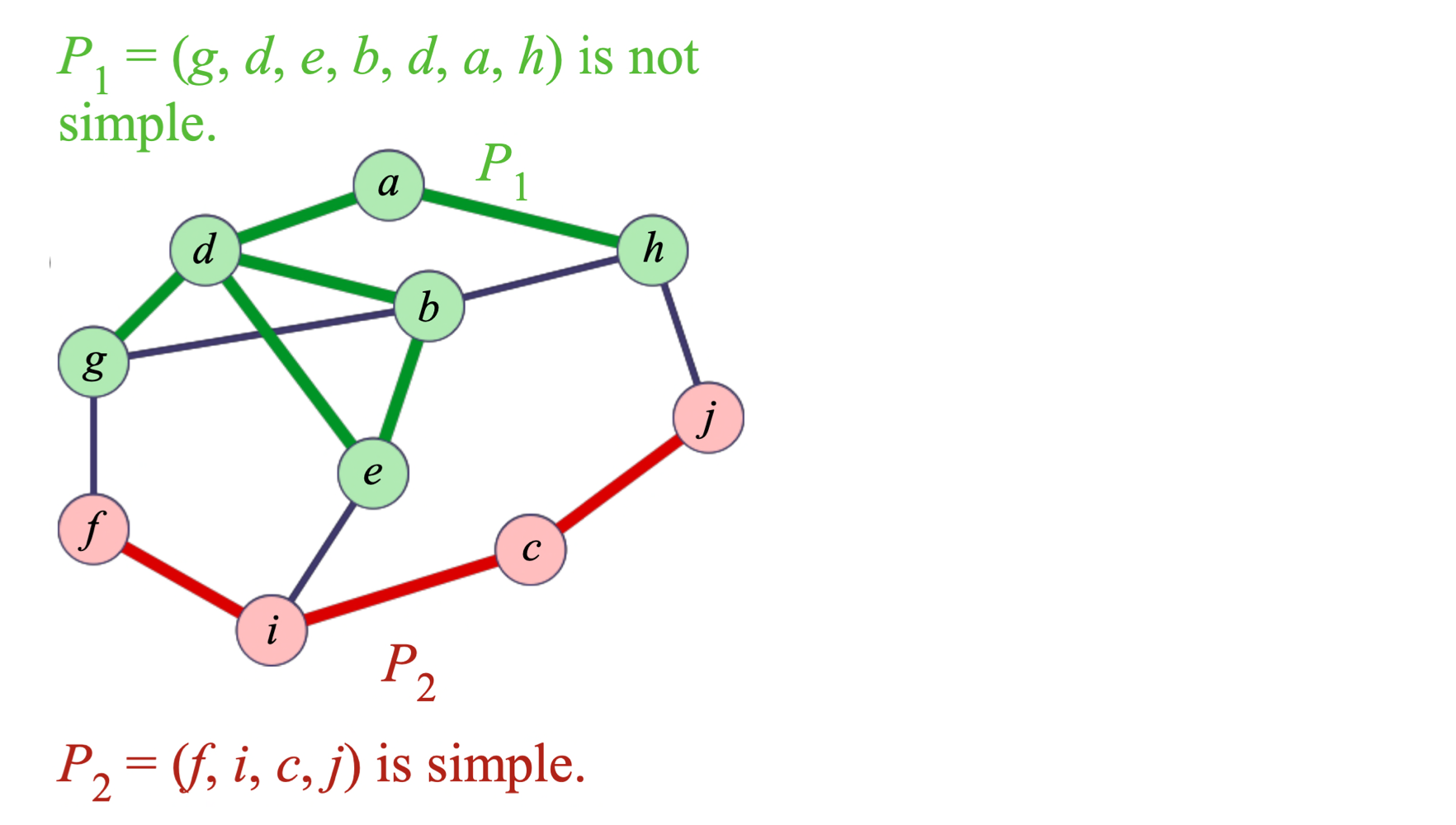 Cycle : a sequence of vertices C = (v, v, ..., v) such that, for 0 ≤ i < k, edge (v, v) ∈ E
Cycle C is simple if the path (v, v, v) is simple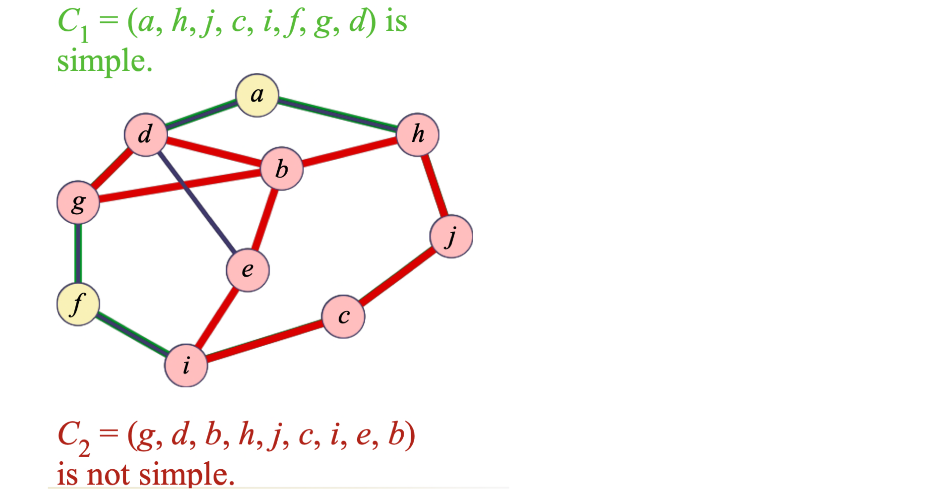 A graph H = (W, F) is a subgraph of a graph G = (V, E)
if W⊆V AND F⊆E
Spanning graph : a subgraph of G that contains all vertices of G
Connectivity : Undirected graph
Connected graph : There is a path between any two vertices in G
Connected components : its maximal connected subgraphs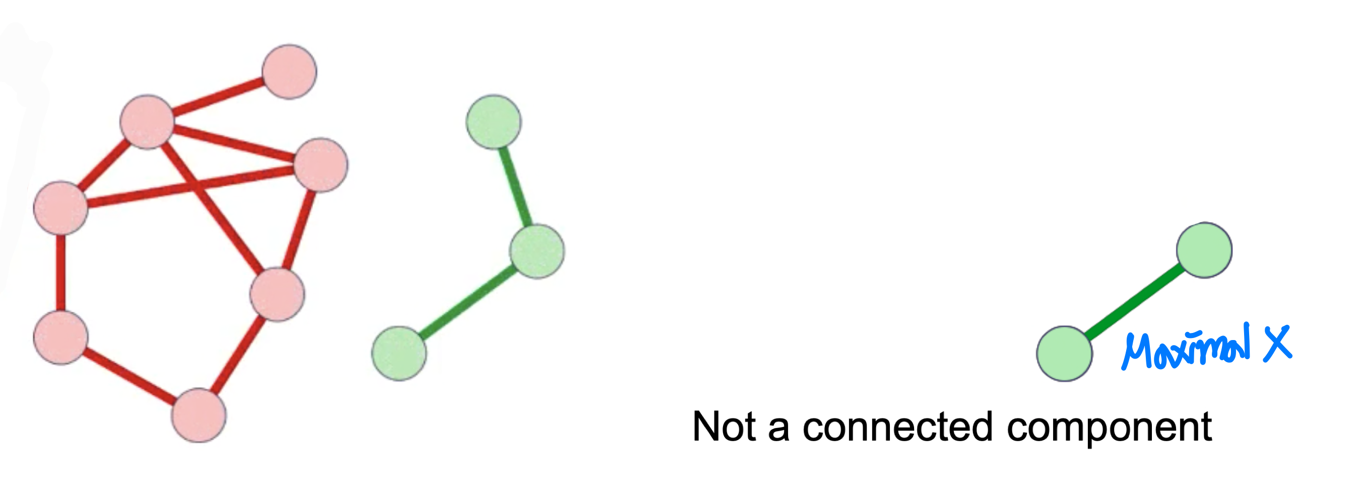 Strongly connected digraph:
- direction affects this!
- node u may be reachable from v, but not v from u ➡️ not strongly connected
- Strongly connected means both directions (Symmetric)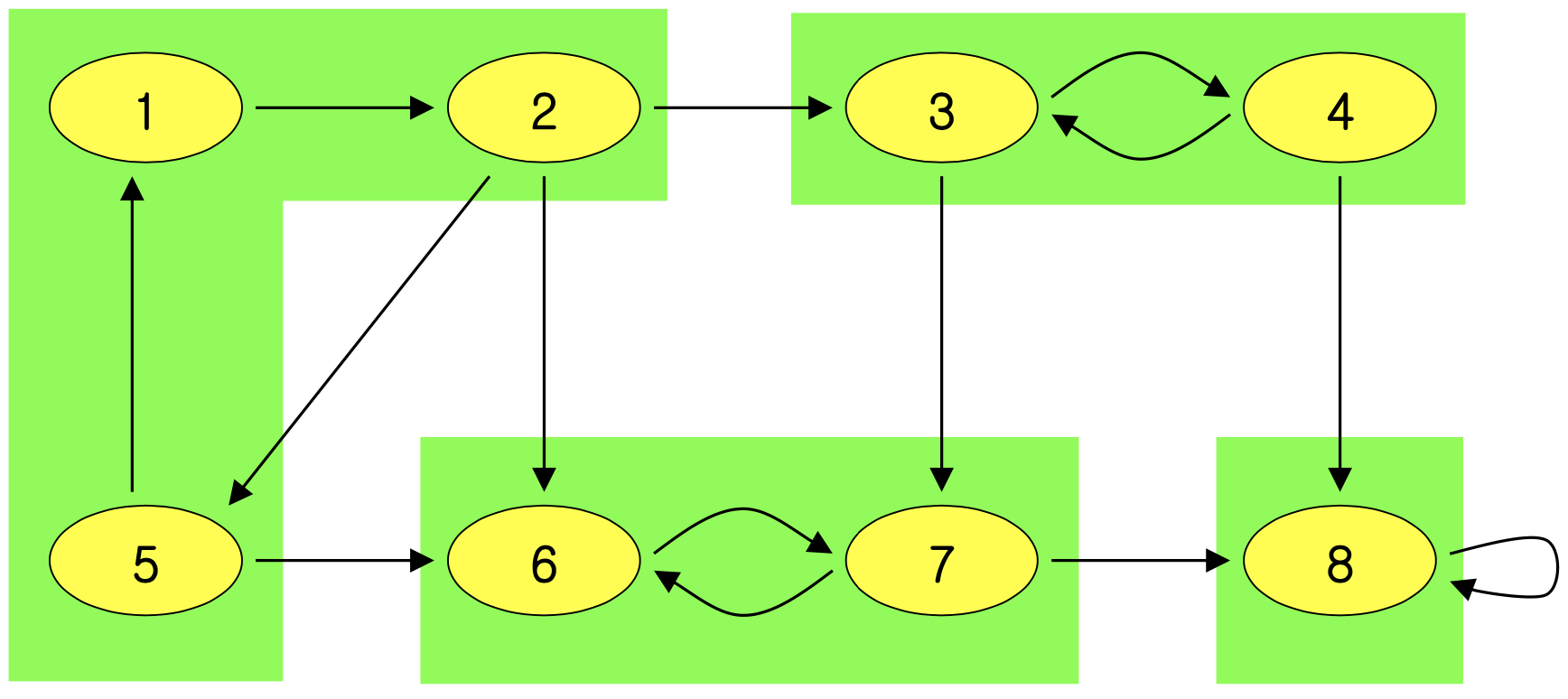 Acyclic: no-cycles
Directed acyclic graph (DAG)
Tree : a graph that is connected and contains no cycles
Spanning tree : Spanning graph + Tree
Adjacency Matrix ➡️ O(V) storage
Q: What is the minimum amount of storage needed by an adjacency matrix representation of an undirected graph with 4 vertices?
A: 6 bits
- Undirected graph ➡️ matrix is symmetric (반대쪽 필요 x)
- No self-loops ➡️ don’t need diagonal (대각선 필요 x)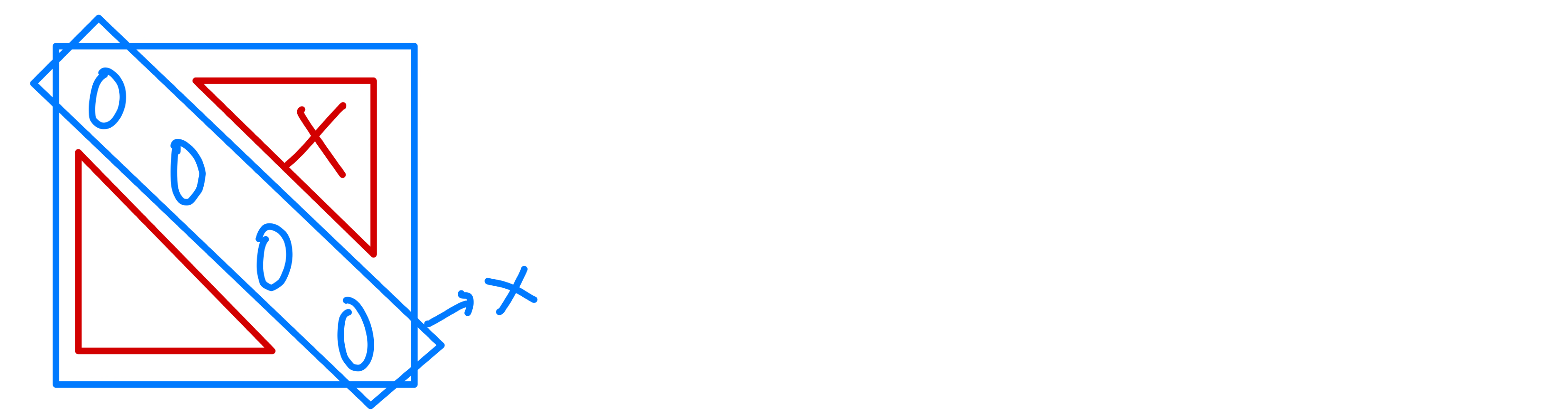
Preferred when the graph is dense
- Usually too much storage for large graphs
- But can be very efficient for small graphs
Most large graphs are sparse
- For this reason the adjacency list is often a more appropriate(적절한) representation
Adjacency List ➡️ O(V+E) storage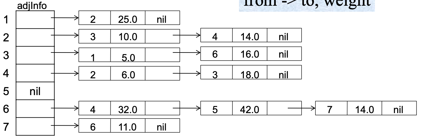
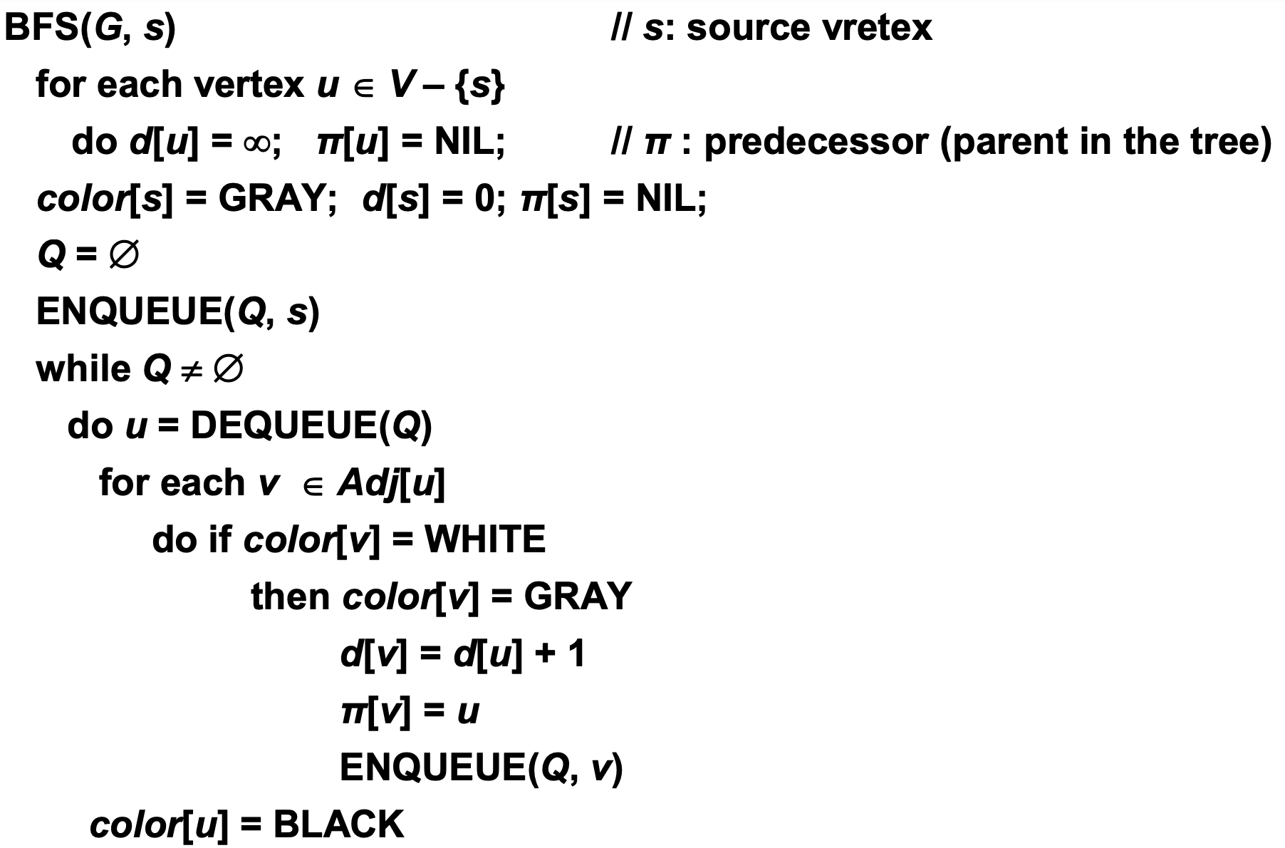
🖥️ BFS
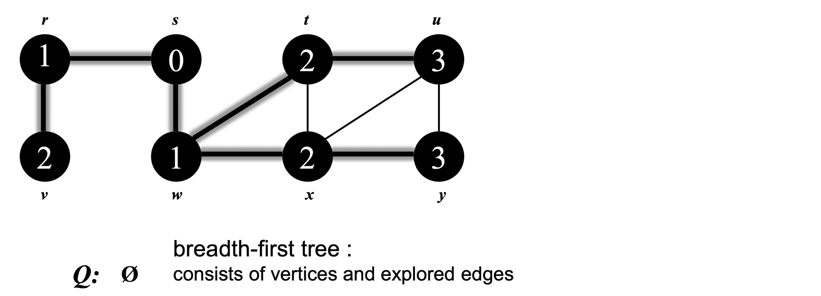
- Scan a graph, and turn it into a 'Breadth-first (spanning) tree'
- Tree with discovered vertices and explored(탐색한) edges
- One vertex at a time
- Pick a source vertex, s to be the root.
- Find(discover) its children, then their children, etc.
- For any vertex reachable from s, the path in the tree from s to v corresponds to a "shortest path" from s to v in G
➡️ ‘Discover’ the vertex : The vertex is first encountered (all vertex)
➡️ ‘Explore’ the edge : The edge is first examined (explore하지 않은 edge 존재 가능)
- White vertices have not been discovered
- All vertices start out white
- Gray vertices are discovered but not finished
- They may be adjacent to white vertices
- The vertex is added to breadth-first tree
- Black vertices are discovered and finished
- They are adjacent only to black and gray vertices
- They are adjacent only to black and gray vertices
- As soon as the white vertex is discovered
- Turn its color to ‘gray’
- Discover all of its white neighbor
- After all of its neighbors are discovered, turn its color to black (means it is finished)
- Discover vertices by scanning adjacency list of gray vertices
Analysis
Running time of Breadth-First search:
A. Each node is enqueued once. (white ➡️ gray) : Θ(V)
B. Each node is dequeued once. (gray ➡️ black) : Θ(V)
C. Each adjacency list is scanned only once. : Θ(E)
➡️ Overall running time is Θ(V+E)
Example
Vertex is an island and edge is an bridge. BFS is visualized as many simultaneous (or nearly simultaneous) explorations from the starting point and spreading out independently.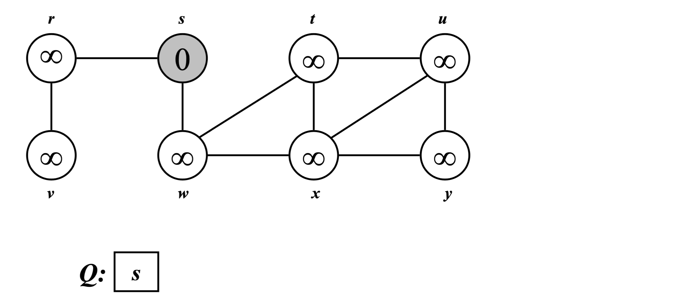
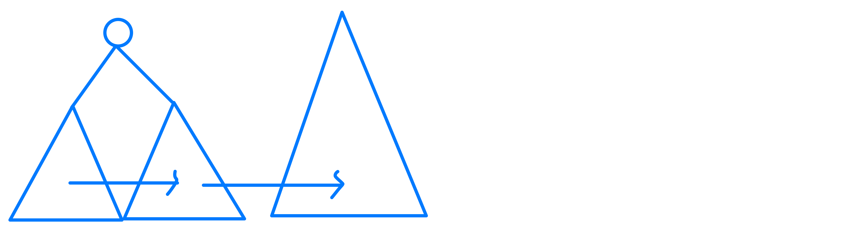
Exercise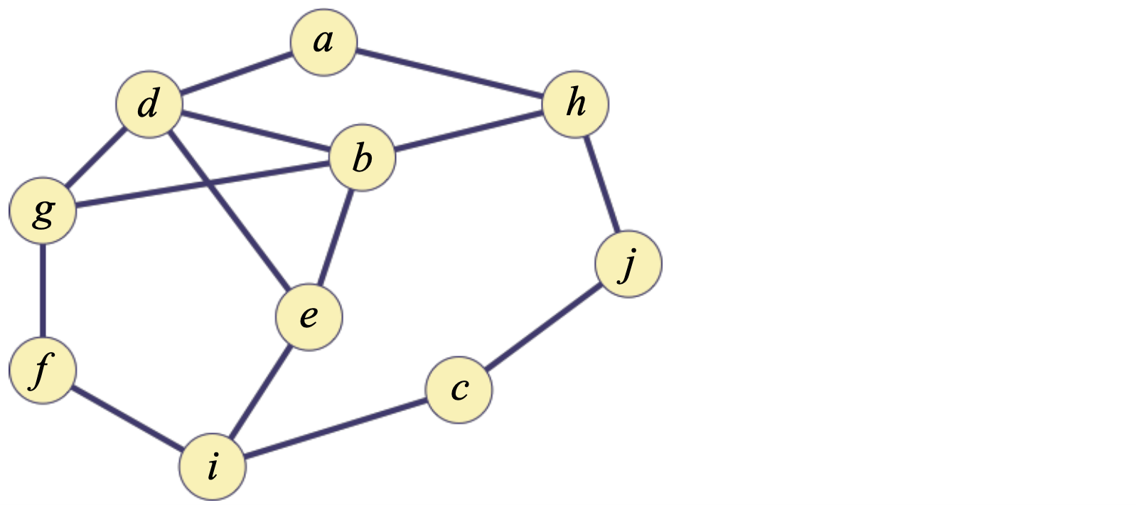
For the following graph,
1) Build breadth-first (spanning) tree with vertex 'a' as root. Assume the vertices are in alphabetical order in the Adj array and that each adjacency list is in alphabetical order
➡️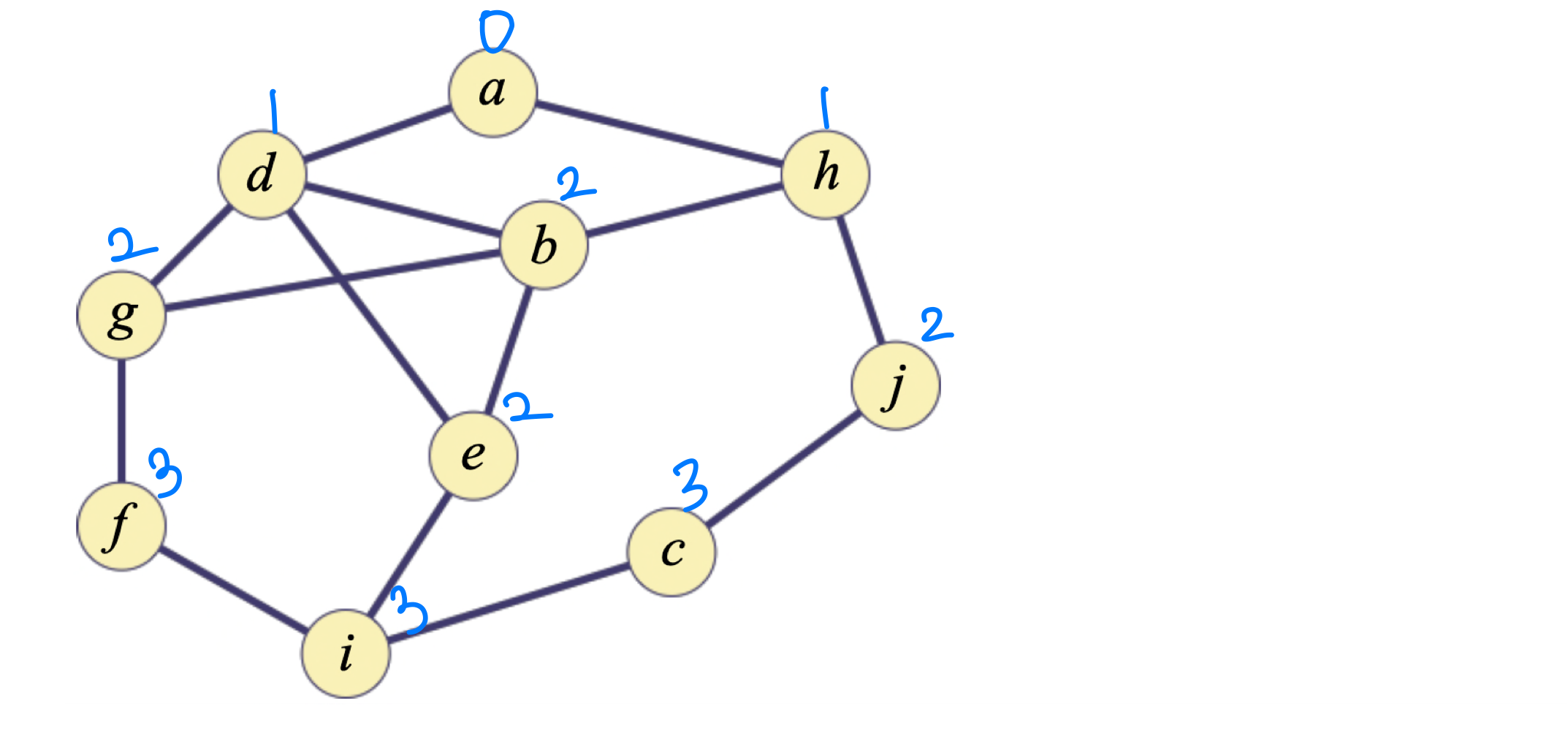
2) What is the minimum distance of vertex c from the root?
➡️ 3
Properties of Breadth-First Search
Theorem: Breadth-first search visits the vertices of G by increasing distance from the root. BFS builds breadth-first tree, in which paths to root represent shortest paths in G
Theorem: For every edge (v, w) in G such that v ∈ L and w ∈ L, | i – j | ≤ 1
➡️ adj vertex와 같거나 1차이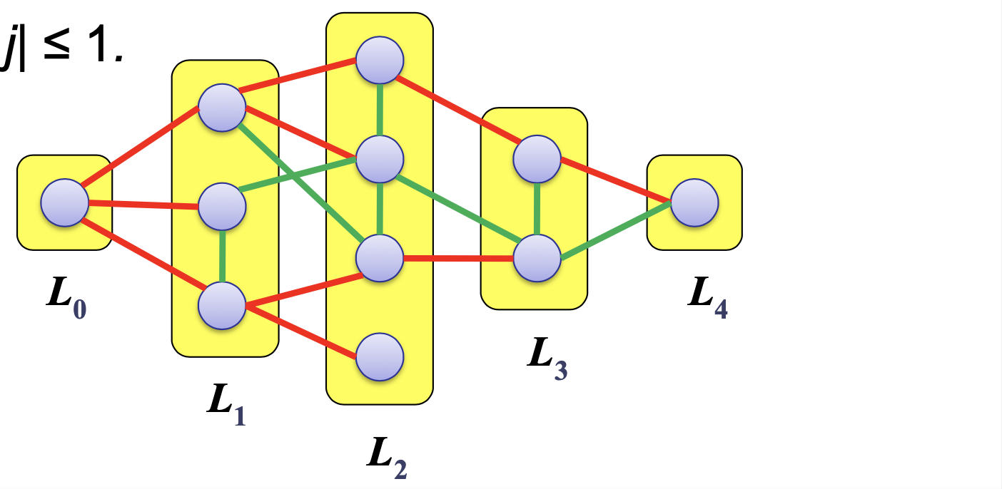
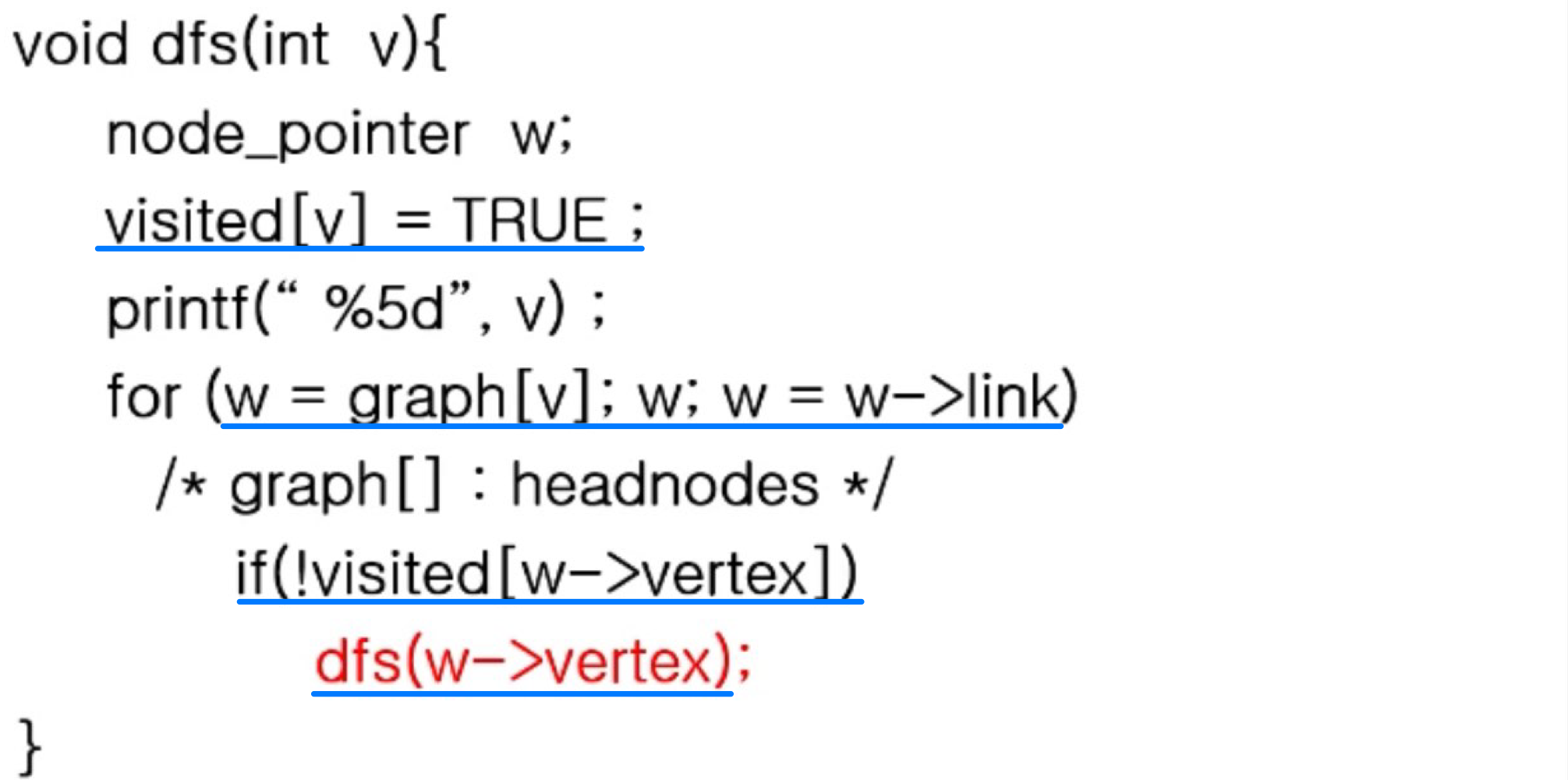
🖥️ DFS
- Depth-first search is another strategy for exploring(모든 vertex를 방문하는 것) a graph
- Explore “deeper” in the graph whenever possible (가능한)
- Pick a source vertex, s to be the root
- Edges are explored out of the most recently discovered vertex v (=deeper) that still has unexplored edges
- When all of v’s edges have been explored, backtrack to the vertex from which v was discovered
- When one dfs tree is finished, start over(다시) from undiscovered vertex as necessary ➡️ Disconnected G
- As soon as we discover a vertex, explore from it. It isn’t like BFS, which puts a vertex on a queue so that we explore from it later.
- When the adjacent vertex is already discovered, the edge is not explored (but checked) ➡️ BFS와 동일
- As DFS progresses, every vertex has a color
- WHITE : undiscovered
- GRAY : discovered, but not finished (not done exploring from it)
- BLACK : finished (have found everything reachable from it)
- Input : G = (V, E), directed or undirected.
- Output : 2 timestamps on each vertex :
- d[v] = discovery time
- f[v] = finish time
- Discovery and finish times :
- Unique integer from 1 to 2|V|
- For all v, d[v] < f[v]
- 1 ≤ d[v] < f[v] ≤ 2|V|

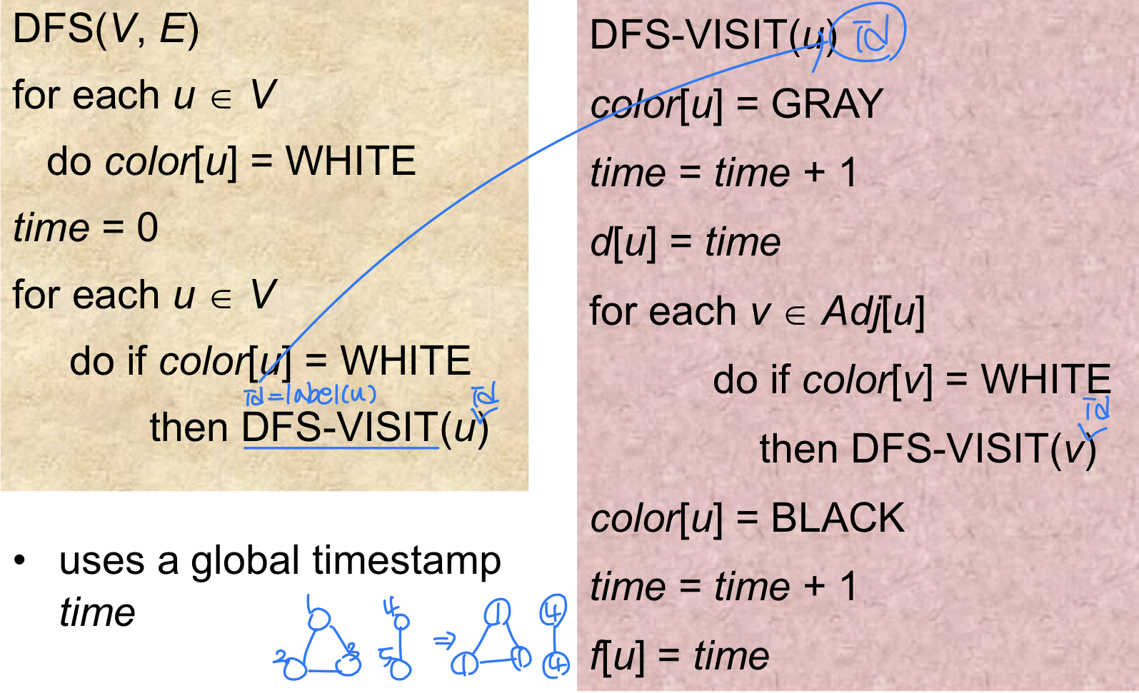
Algorithm
DFS(V, E)
for u : V
color[u] = WHITE
time = 0 // Global timestamp
for u : V
if color[u] == WHITE
DFS-VISIT(u)
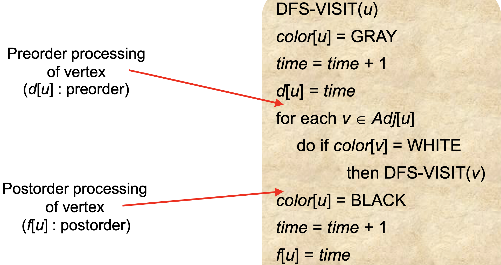
DFS-VISIT(u)
// Discovery
color[u] = GRAY
time++
d[u] = time
// Adj
for v : Adj[u]
if color[v] == WHITE
DFS-VISIT
// Finish
color[u] = BLACK
time++
f[u] = time
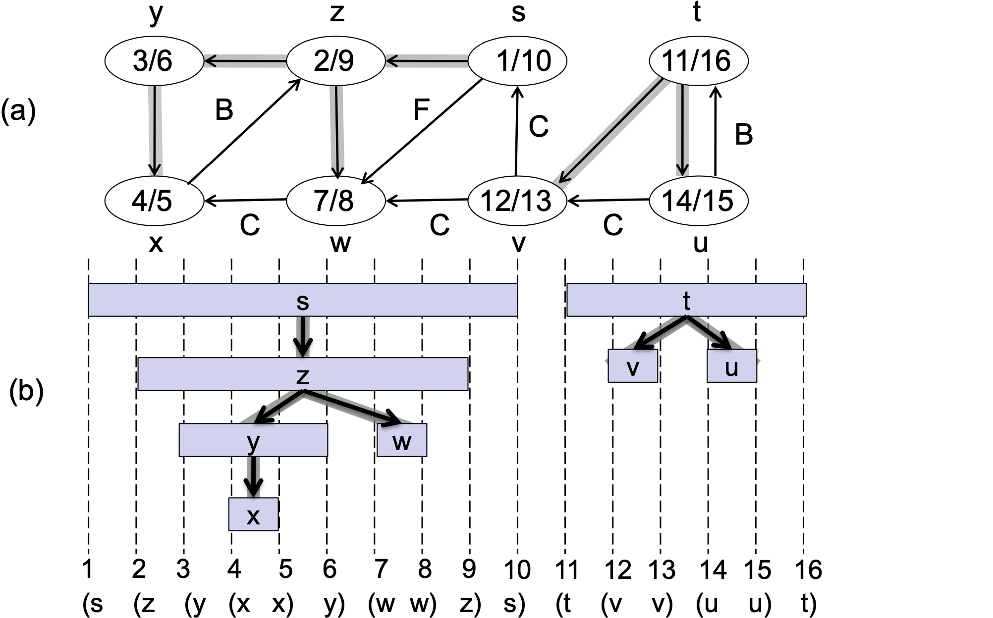
Example
One person(동시X) explores the islands. If an island is not discovered yet, walk in the direction as arrows. If one walk across the bridge in the reverse direction, one should walk backward – backtracking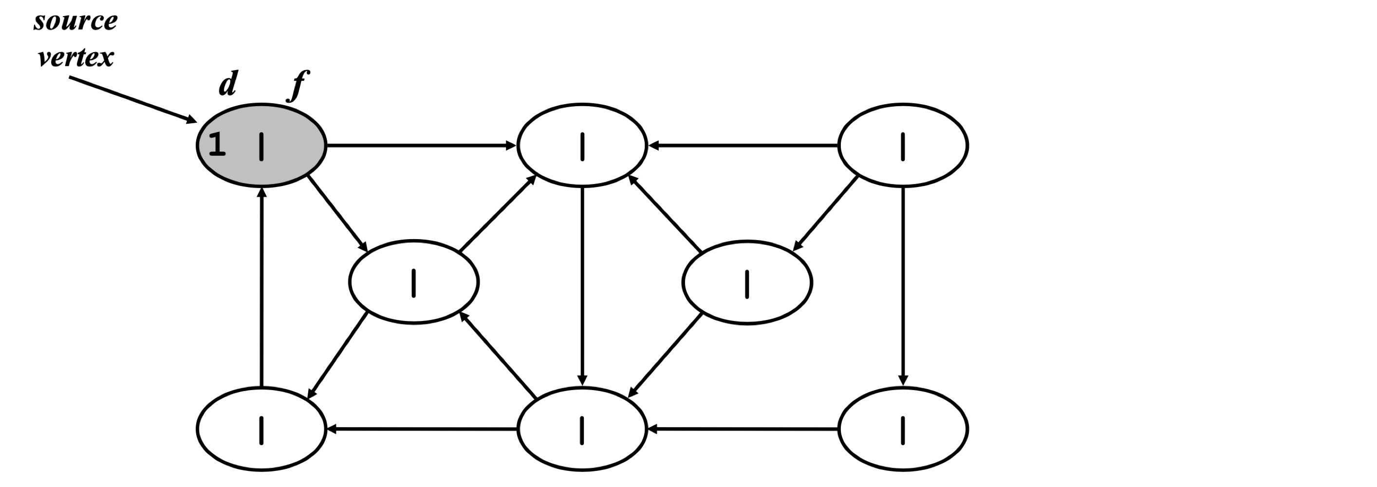
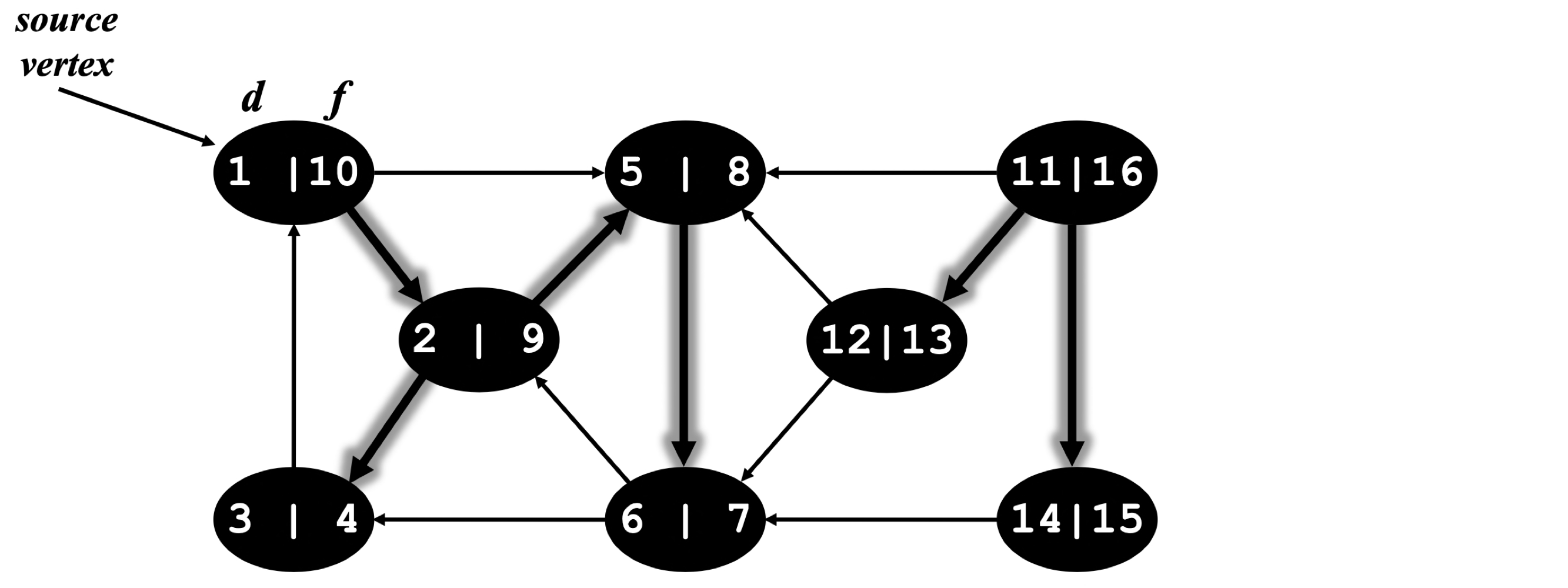
Exercise
Assume the vertices are in alphabetical order in the Adj array and that each adjacency list is in alphabetical order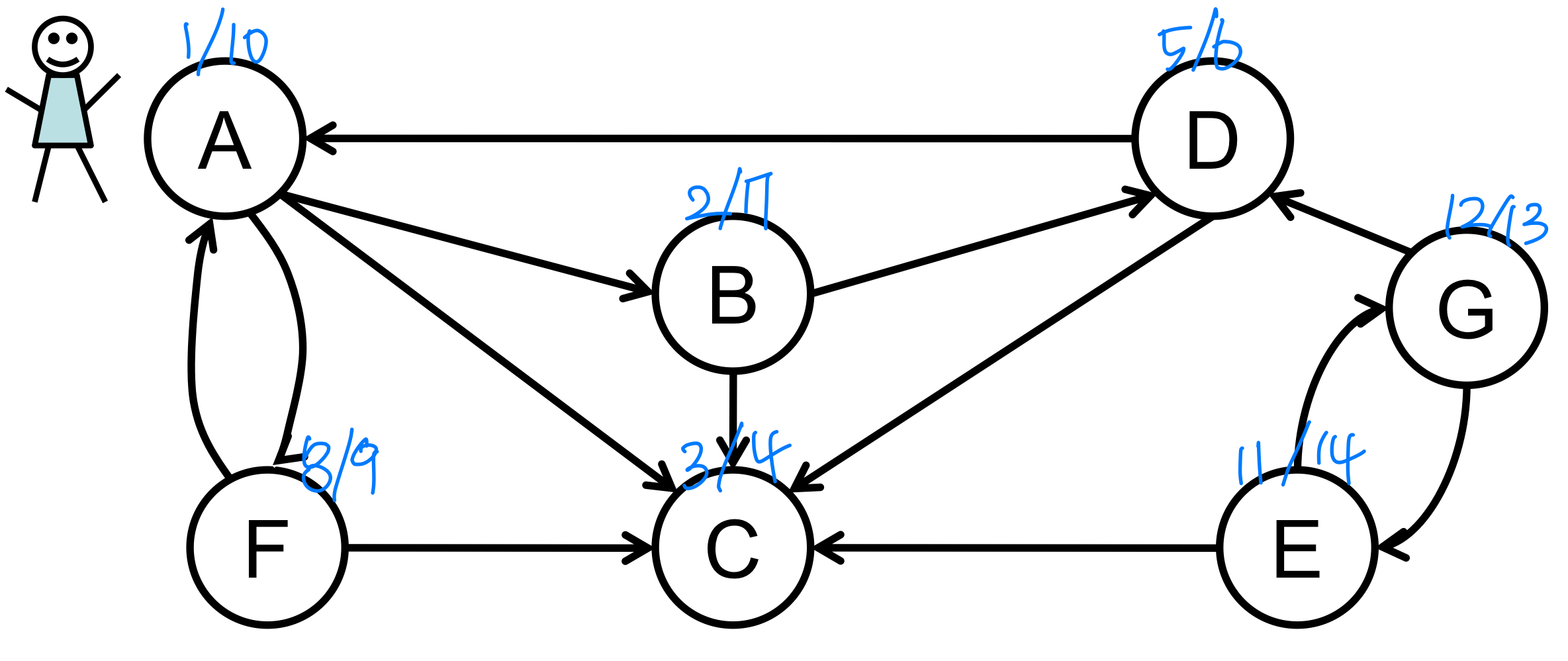
Analysis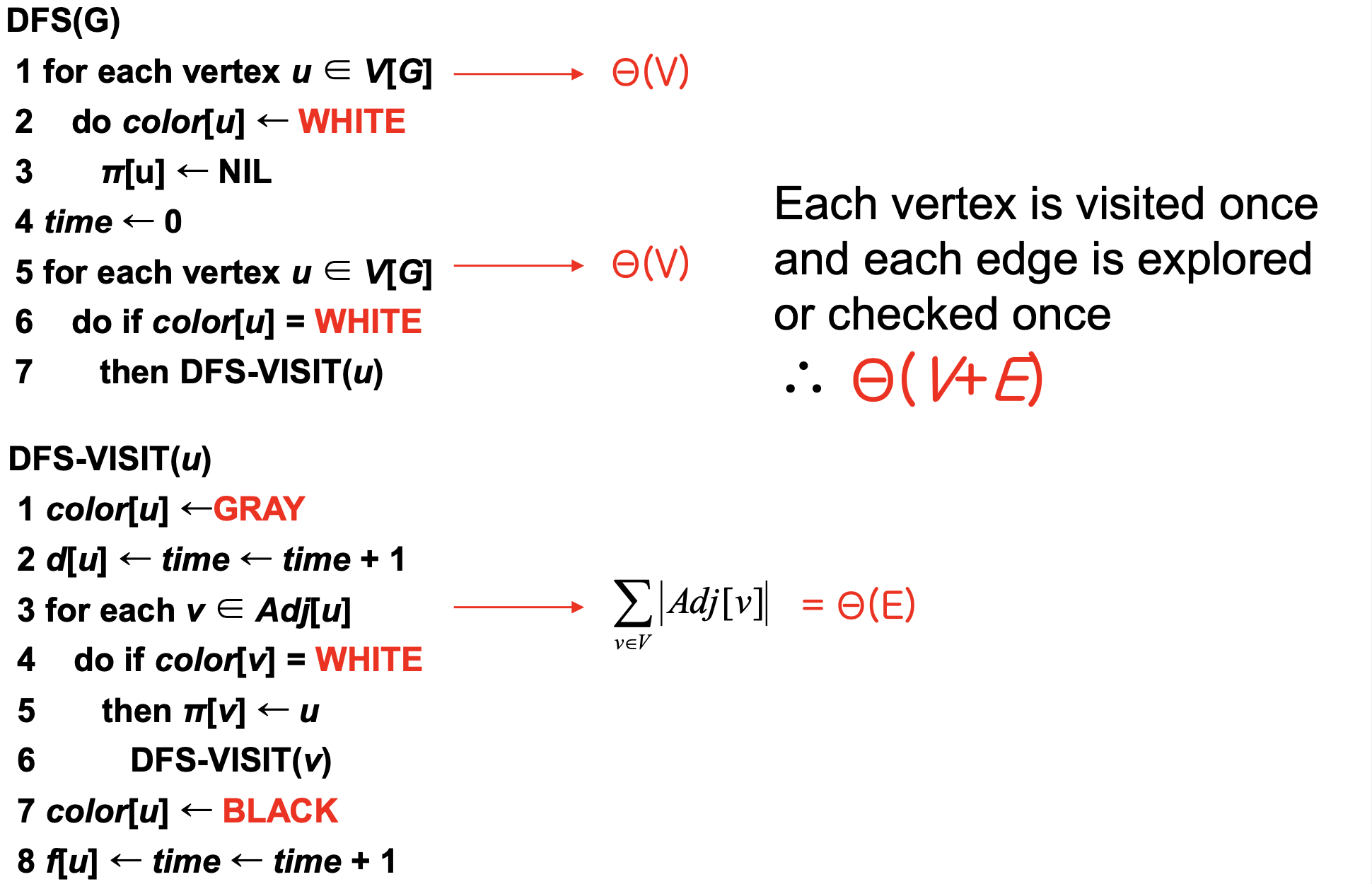
- DFS on tree vs. general graph
- G1, G2, G3 are disjoint set, so we don’t have to worry about the possibility of visiting node already visited
- Edge in a tree is one way, i.e. no cycle ➡️ |V| = n, |E| = n-1
Parenthesis theorem
For all u, v, exactly one of the following holds :
1. d[u] < f[u] < d[v] < f[v] or d[v] < f[v] < d[u] < f[u] and
neither of u and v is a descendant(child) of the other
2. d[u] < d[v] < f[v] < f[u] and v is a descendant of u
3. d[v] < d[u] < f[u] < f[v] and u is a descendant of v
➡️ So d[u] < d[v] < f[u] < f[v] cannot happen
Like parentheses :
()[] , ([]), [()] are O.K, but ([)][(]) are not O.K
Corollary :
v is a proper descendant of u if, d[u] < d[v] < f[v] < f[u]
Proof
Assume that d[u] < d[v] (because of symmetry)
1️⃣ d[v] < f[u]
v was discovered while u was gray, and this implies that v is a descendant of u. Moreover, since v was discovered more recently than u, all of its outgoing edges are explored, and v is finished, before the search returns to and finishes u
So, f[v] < f[u]
∴ d[u] < d[v] < f[v] < f[u]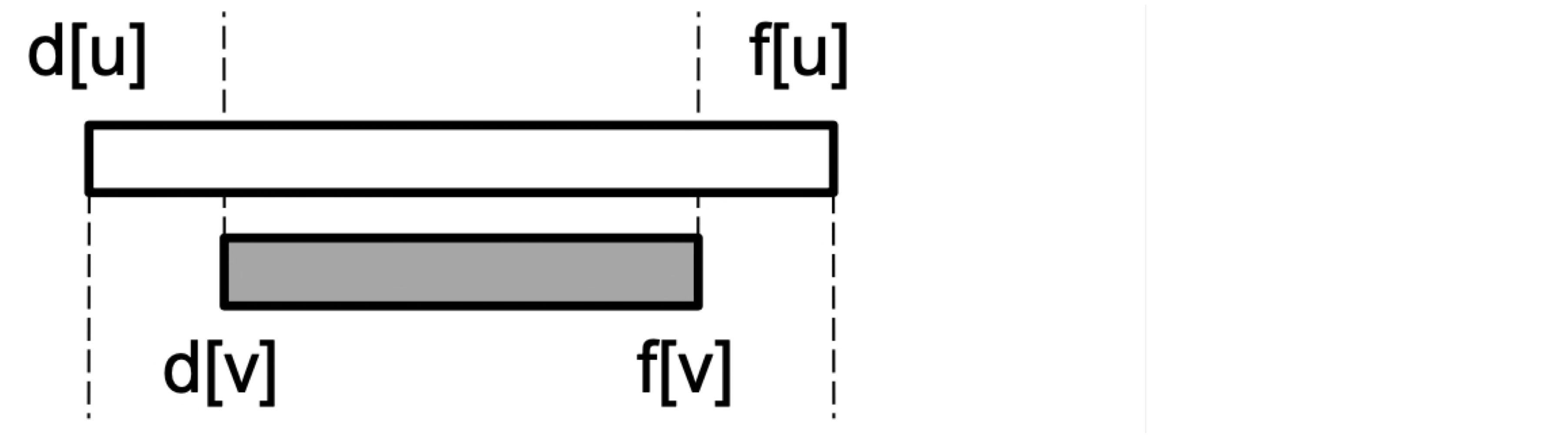 Thus, the interval(구간) [d[v],f[v]] is entirely(완전히 포함) contained within the interval [d[u],f[u]]
2️⃣ d[v] > f[u] (disjoint intervals)
∴ d[u] < f[u] < d[v] < f[v]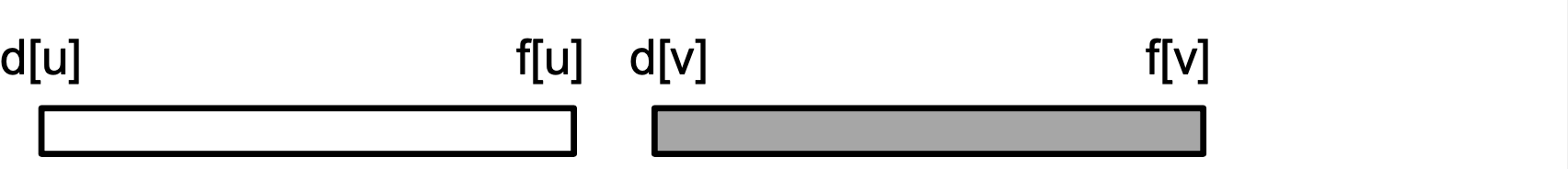
DFS : Kinds of edges
- Tree edge: encounter new (white) vertex
- The tree edges form a spanning forest (explored)
- Can tree edges form cycles? ➡️ No
Why or why not?
- Back edge: from descendent(child) to ancestor(parent) (checked)
- Encounter a gray vertex (gray to gray)
- Encounter a gray vertex (gray to gray)
- Forward edge: from ancestor to descendent (checked)
- Not a tree edge, though
- From gray node to black node
- Cross edge: between a tree or subtrees (checked)
- From a gray node to a black node
- From a gray node to a black node
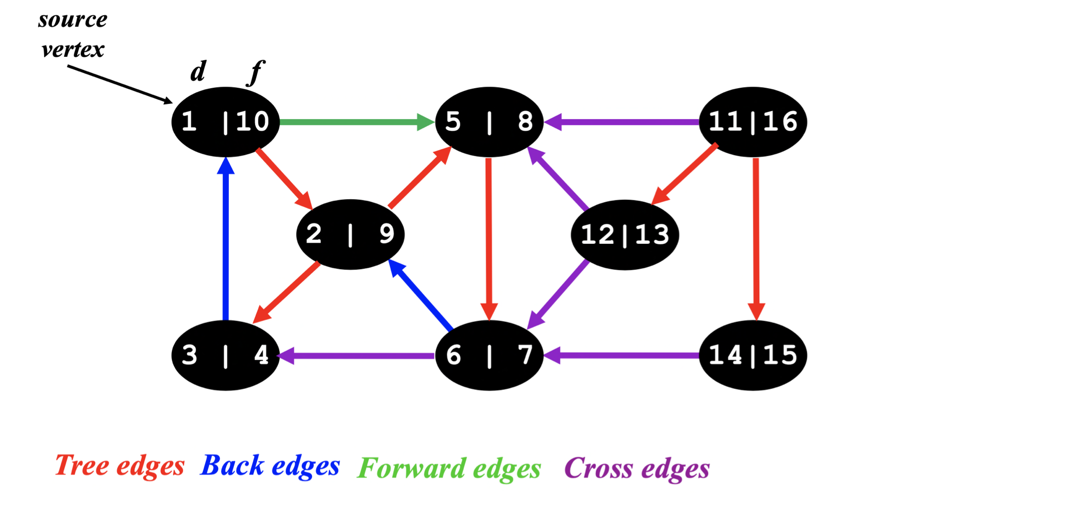
Example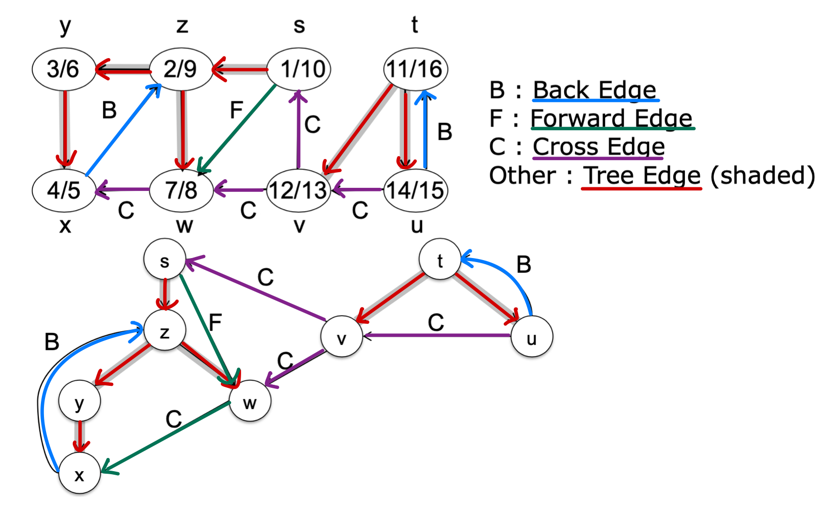
- From a gray node to a white node
➡️ tree edge - From a gray node to a gray node
➡️ back edge - From a gray node to a black node
➡️ forward or cross edge - Then how do you tell(구분) the forward edge from cross edge?
➡️ Discovery, finish time으로- forward edge
- cross edge
- forward edge
DFS on Undirected graph
- If it doesn’t matter if an edge is processed twice
- transform it into symmetric digraph, then process edge twice
- Else
- edge should be explored in one direction. The direction is determined when the edge is first encountered

- edge should be explored in one direction. The direction is determined when the edge is first encountered
DFS : Kinds of Edges continue
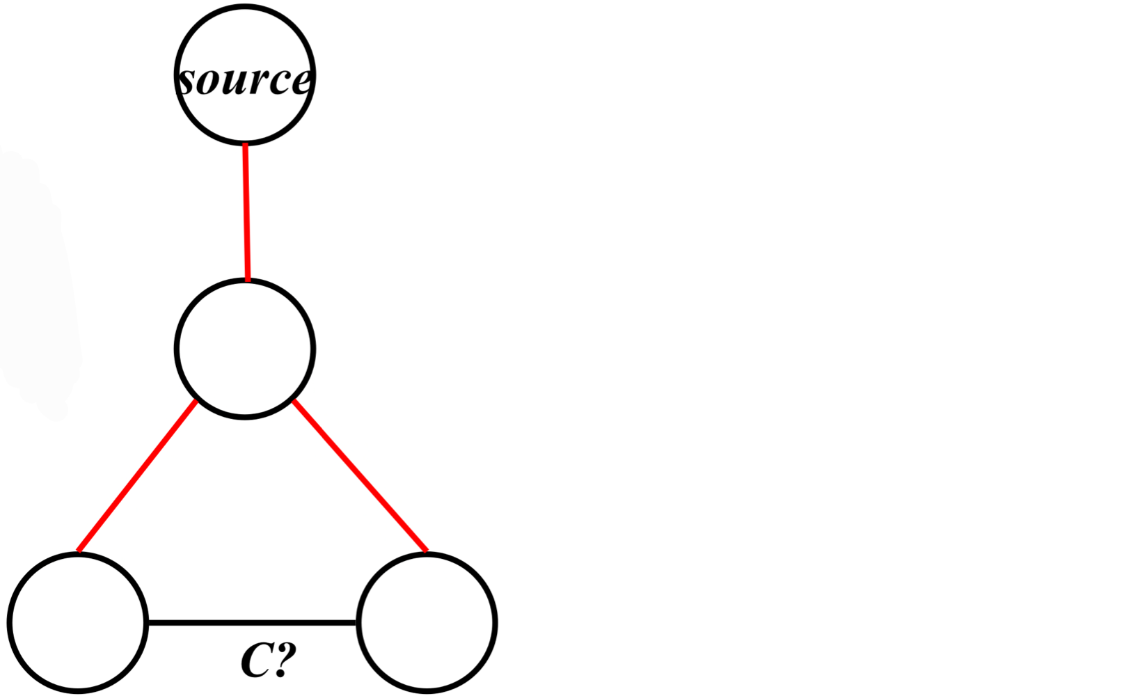
- Theorem 22.10: If G is undirected, a DFS produces only tree and back edges ( cross / foward X )
- Proof by contradiction:
- Assume there’s a forward edge
- But F? edge must actually be a back edge (why?)
- It means that the edge is not checked from vertex v
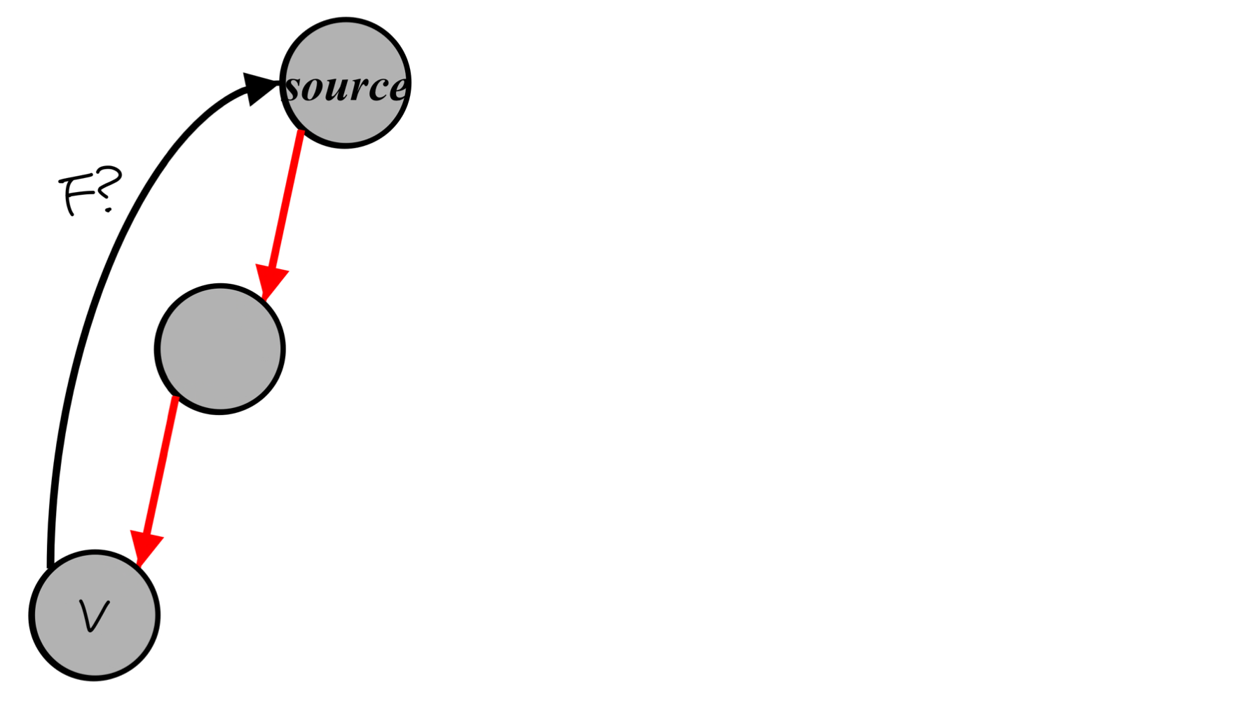
- Assume there’s a cross edge
- But C? edge cannot be cross:
- It should be explored from one of the vertices it connects, becoming a tree vertex, before other vertex is explored
- So in fact the picture is wrong. The lower edge cannot be cross edge, but tree edge
- Assume there’s a forward edge
DFS vs. BFS
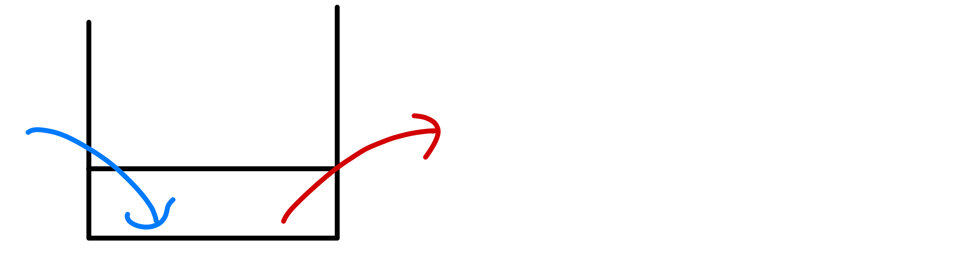
- DFS : Stack
- BFS : Queue
- DFS : Two processing opportunity
- Once when it is discovered(처음 발견했을 때) : Preorder
- Once when it is marked finished : Postorder
- Postorder : We have information about adjacent vertices
 ex) Counting the number of leaves in binary tree
- BFS : One processing opportunity
🖥️ Applications of DFS
1) Topological Sort (DAG)
- Linear ordering (cycle이 없기 때문) of all vertices in graph G such that vertex u comes before vertex v if edge (u, v) G
- Real-world example: getting dressed
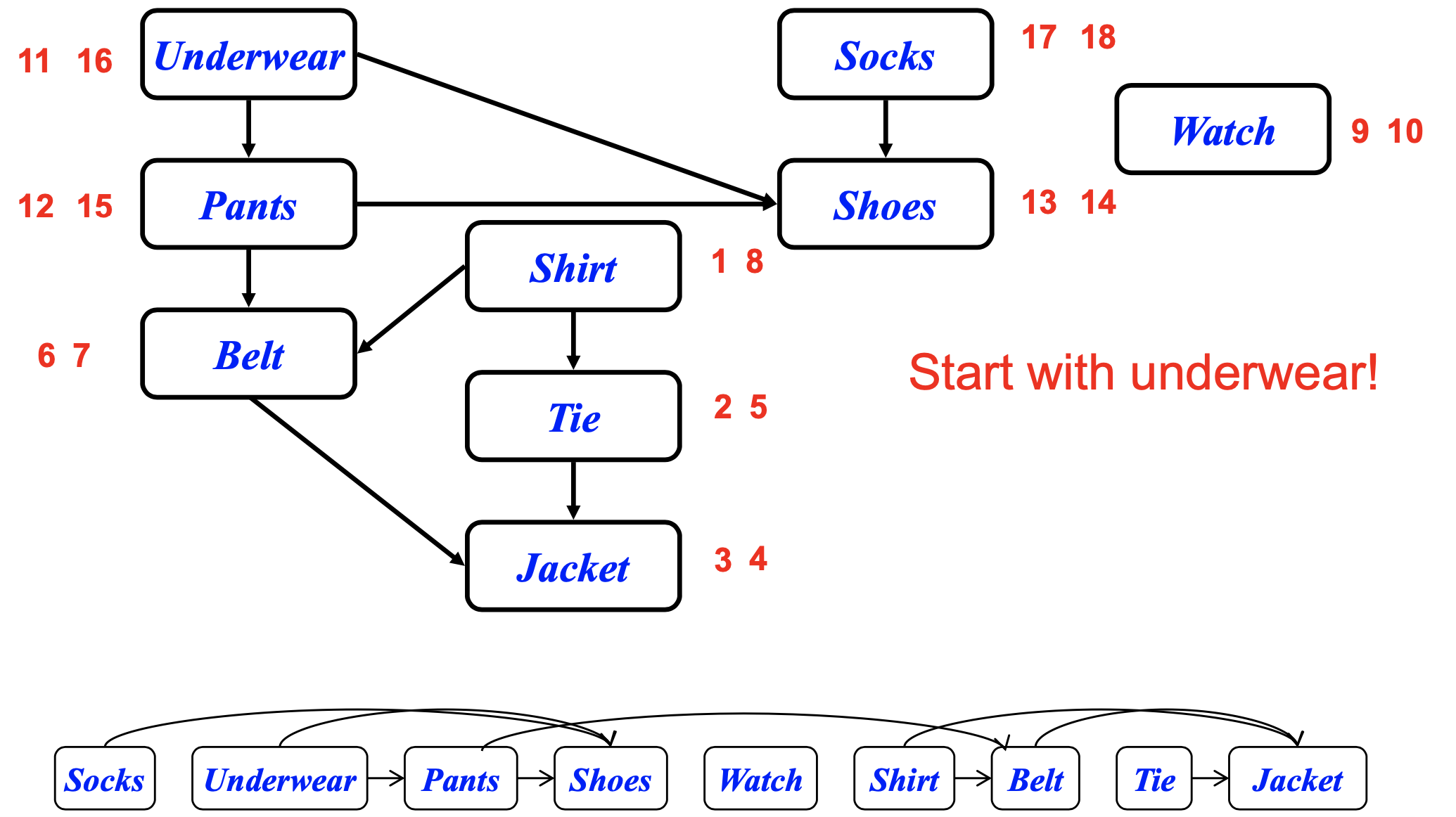 ➡️ Try "Start with underwear
Algorithm
- Topological-Sort()
1. Run DFS to compute finishing times f[v] for all v V ➡️ (V+E)
2. As each vertex is finished, insert it into the front of a linked list (Or output vertices in order of decreasing finish time) ➡️ (V) - Time: Θ(V+E)
- Correctness: Want to prove that (u,v) G ➡️ f[u] > f[v] (finish time)
- When (u,v) is explored, u is gray
- v = gray ➡️ (u,v) is back edge. Contradiction (Why?)
We are dealing with DAG (no cycle) here
- v = white ➡️ v becomes descendent of u ➡️ f[v] < f[u]
(since must finish v before backtracking and finishing u)
- v = black ➡️ v already finished ➡️ f[v] < f[u]
- When (u,v) is explored, u is gray
2) Connected Component (Undirected)
- Convert undirected graph into symmetric graph
- Function DFS (BFS도 가능)
- Find undiscovered vertices and initiate a DFS-VISIT at each undiscovered vertex.
- Pass id – label(v) – of undiscovered vertex v to DFS-VISIT.
- Function DFS-VISIT
- Determine the label of current vertex as label(v) and pass it to its white adjacent vertices.
- Make a separate linked list for each component
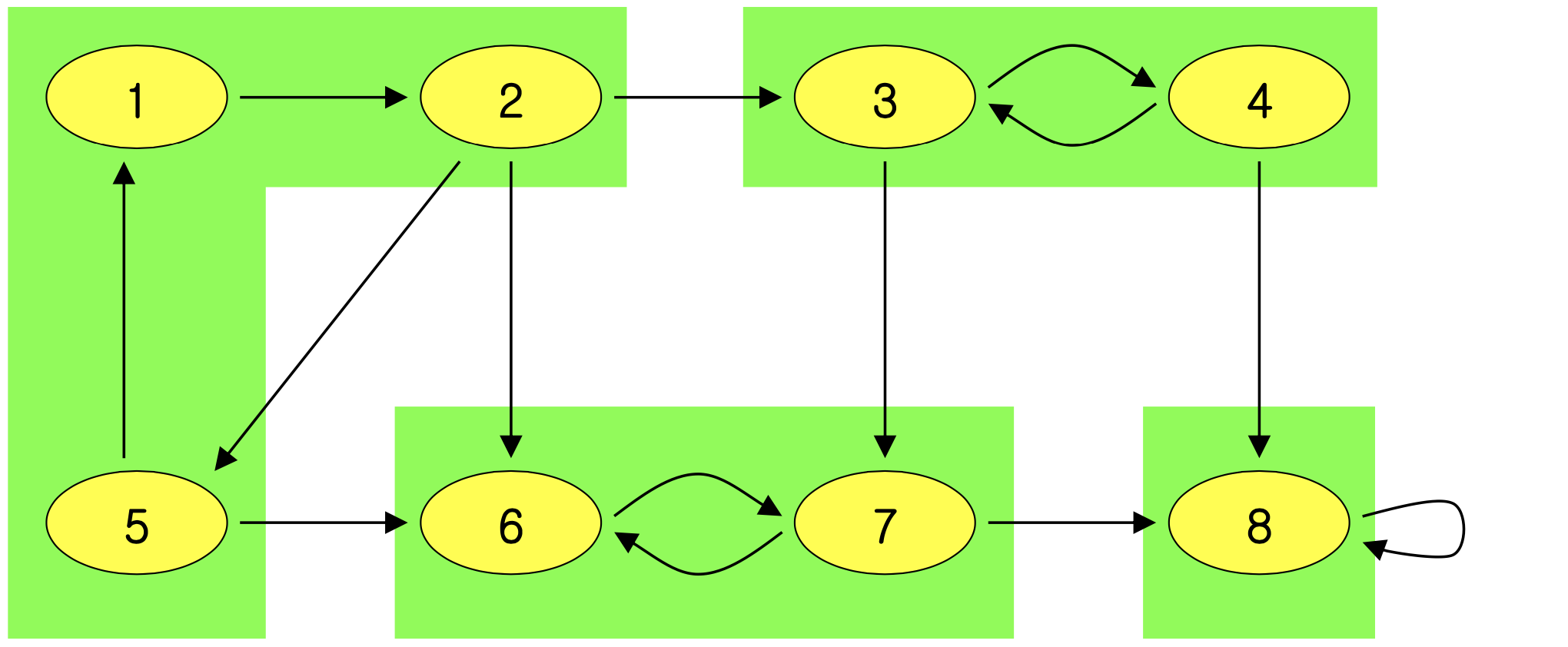
3) Strongly Connected Component (Directed)
- Definition: a maximal set of vertices C ⊆ V such that that for every pair of vertices u and v in C, u → v and v → u
- Informally, a maximal sub-graph in which every vertex is reachable(도달가능) from every other vertex
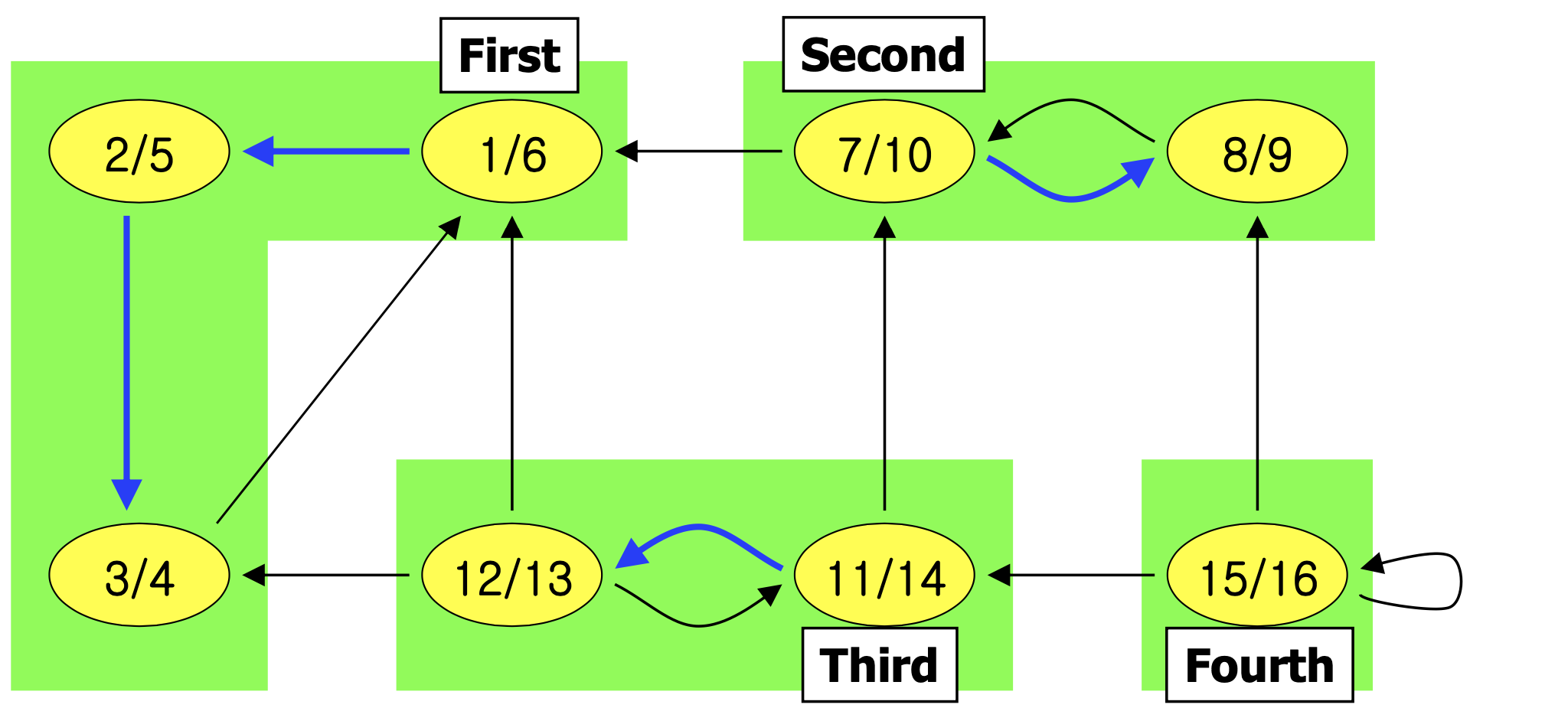
- Example - Green areas are the SCC (4 SCC)
Property
- G and G have exactly the same strongly connected components
- The component graph G is directed acyclic graph(DAG)
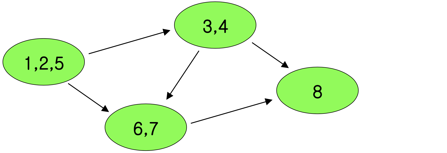 ➡️ cycle이 있다면 cycle components 전체가 SCC
Algorithm
- STRONGY-CONNECTED-COMPONENTS(G)
1. call DFS(G) to compute finishing times f[u] for each vertex u ➡️ (V+E)
2. compute G ➡️ matrix면 (V), list면 (V+E)
3. Call DFS(G), but in the main loop of DFS, consider the vertices in order of decreasing f[u] (not alphabetic) (as computed in line 1) ➡️ (V+E)
4. Output the vertices of each tree in the depth-first forest formed in line 3 as a separate strongly connected component ➡️ (1)
∴ The running time of this algorithm is Θ(V+E)
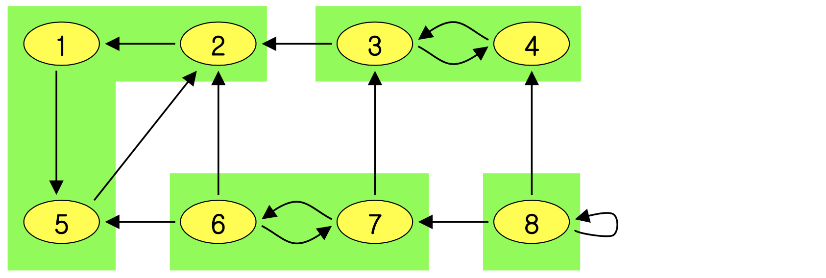
G vs. transpose of G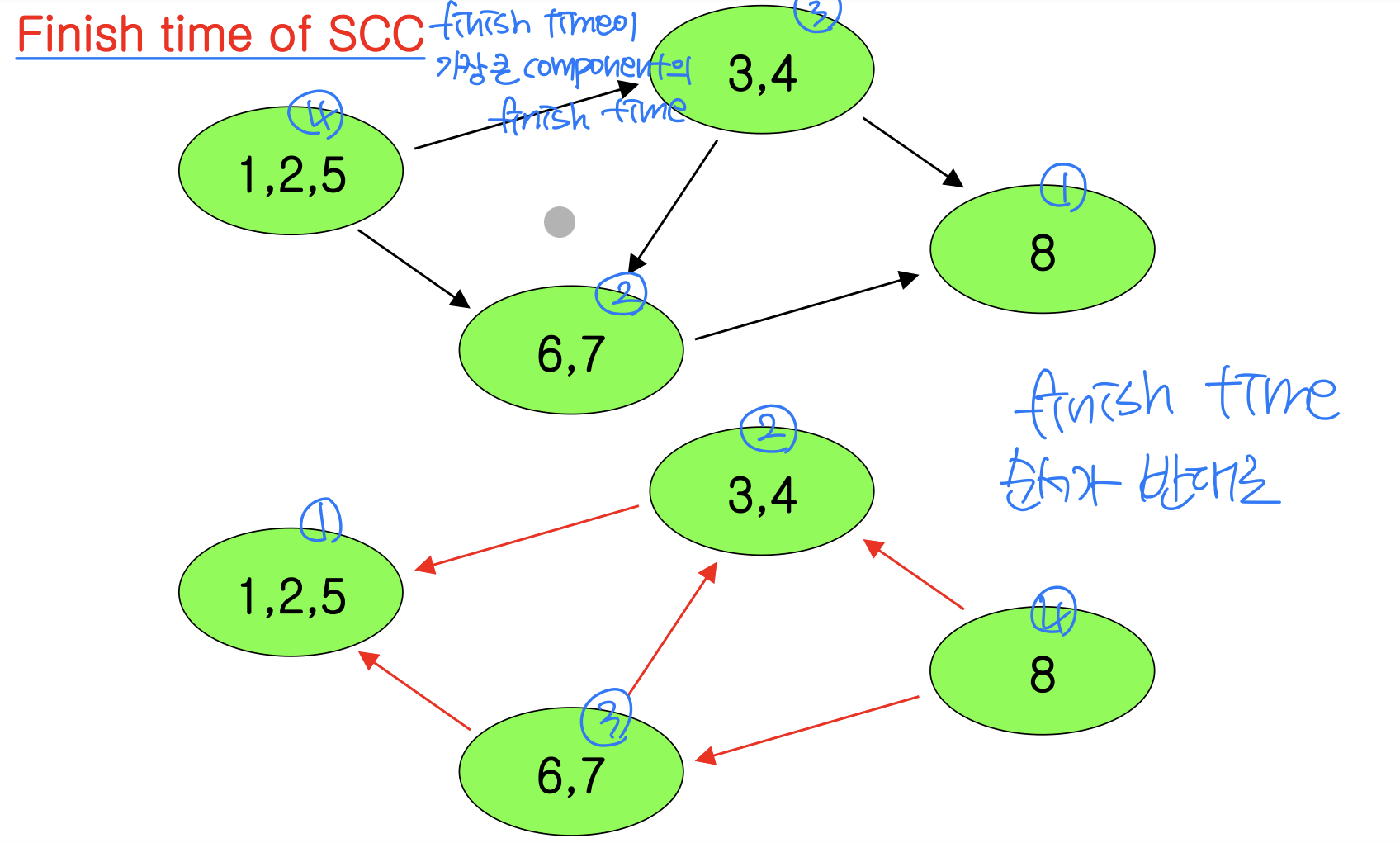
Example
- Step1 : Call DFS(G)
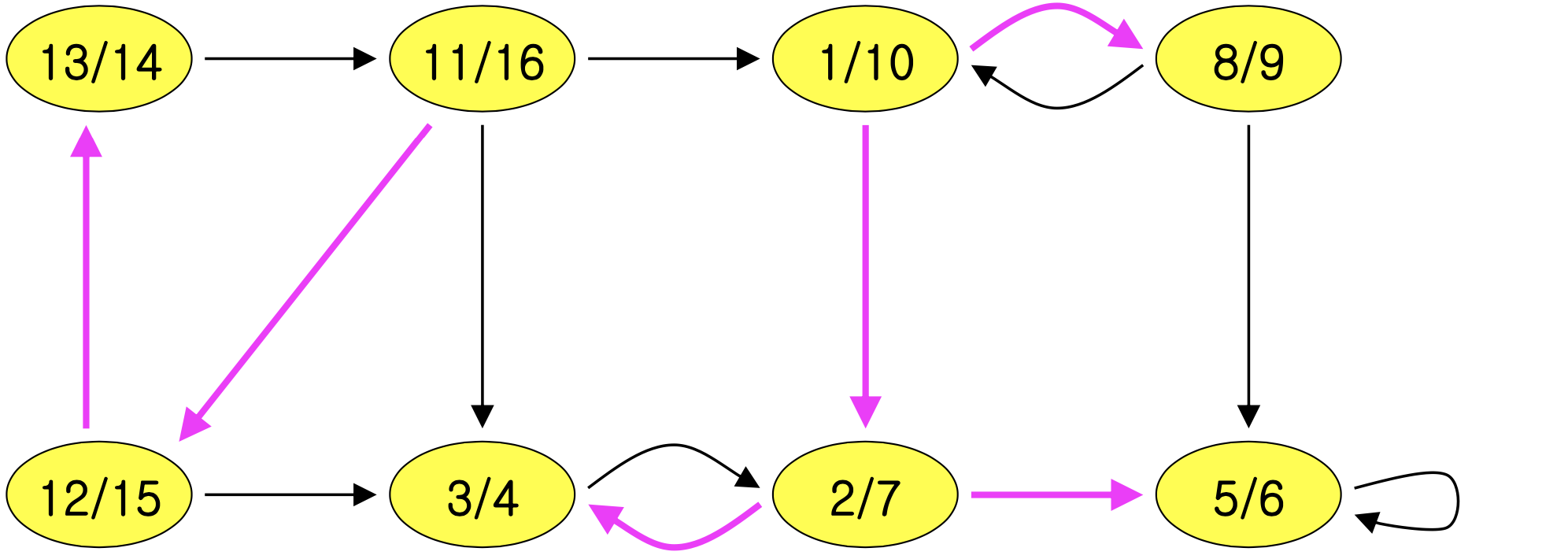
- Step2 : Compute transpose of G
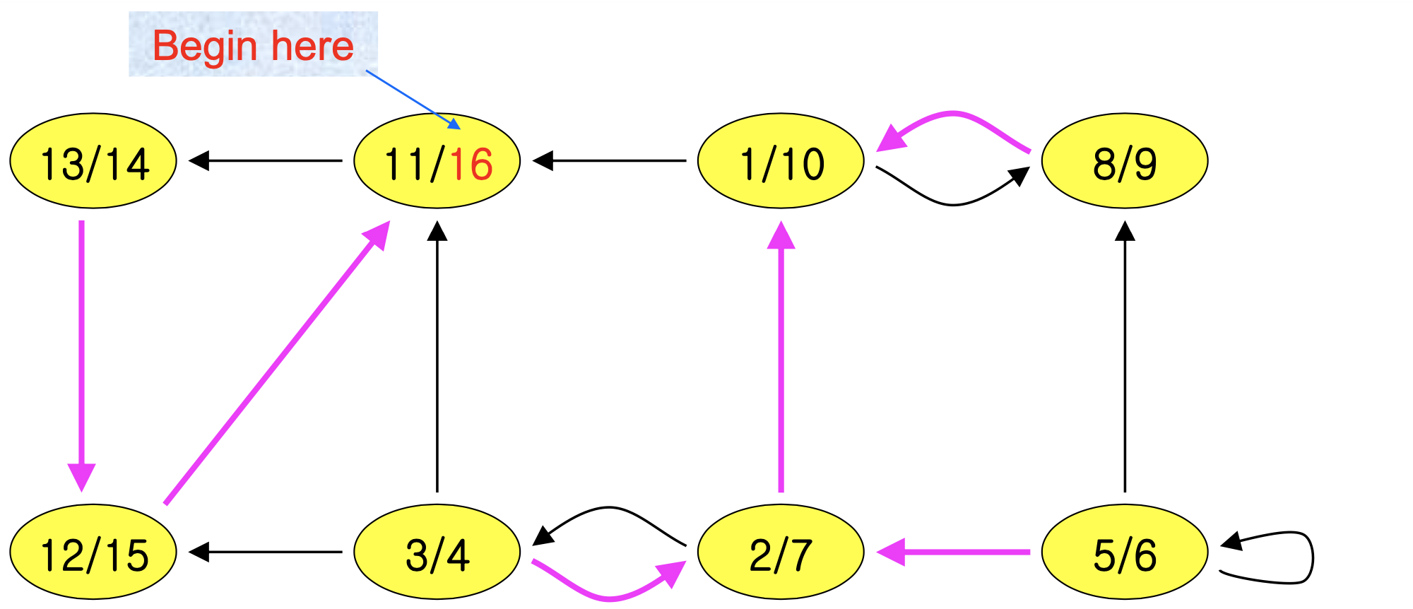
- Step3 : Compute DFS(G), but in order of decreasing f[u]
Lemma and Corollary
- Lemma 22.13
Let C and C’ be distinct strongly connected components in directed graph G = (V, E), let u, v ∈ C, let u’, v’ ∈ C’, and suppose that there is a path u → u’ in G. Then there cannot also be a path v’ → v in G
- Lemma 22.14
Let C and C’ be distinct strongly connected components in directed graph G = (V, E). Suppose that there is an edge (u, v) ∈ E, where u ∈ C and v ∈ C’. Then f(C) > f(C’)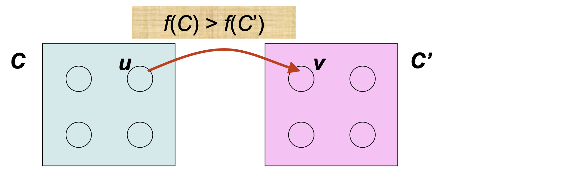
- f(U) = max {f [u]}(가장 큰 finish time의 component). That is f(U) is latest finishing time of any vertex in U
- f(U) = max {f [u]}(가장 큰 finish time의 component). That is f(U) is latest finishing time of any vertex in U
- Corollary 22.15
Let C and C’ be distinct SCC’s in G = (V, E). Suppose there is
an edge (v,u) ∈ E, where u ∈ C and v ∈ C’. Then f(C) > f(C’)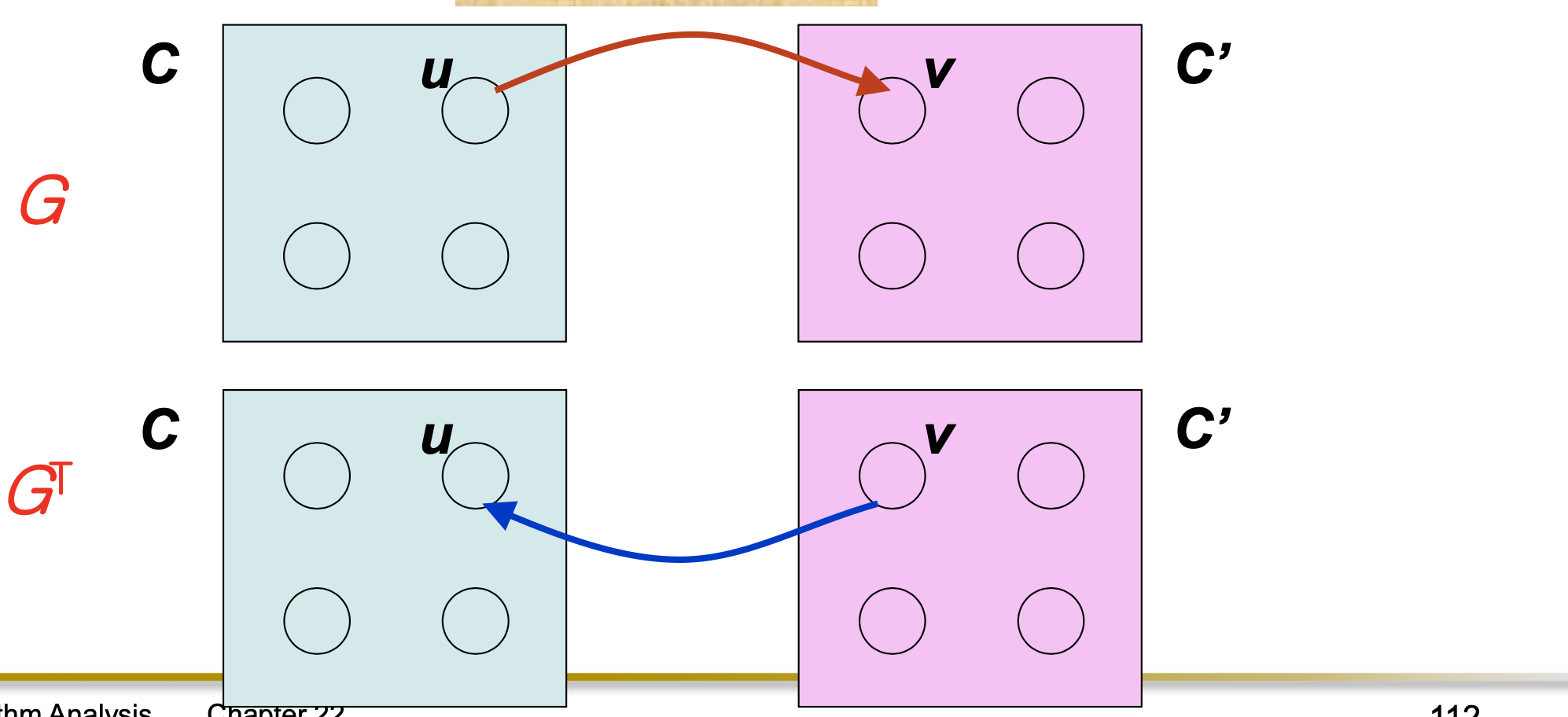
- Corollary
Let C and C’ be distinct SCC’s in G = (V, E). Suppose that f(C) >f(C’). Then there cannot be an edge from C to C’ in G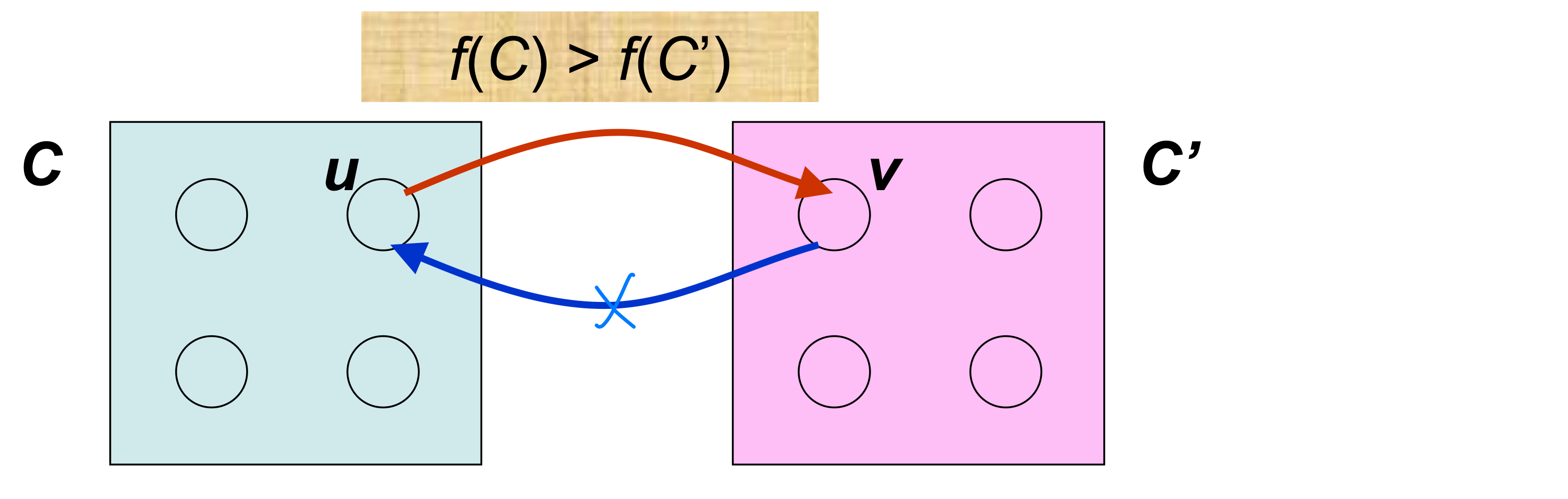
Theorem
- Theorem 22.16
STRONGLY-CONNECTED-COMPONENTS(G)
correctly computes the strongly connected components of a directed graph G
- When we do 2nd DFS on G, start with SCC C s.t. f(C) is maximum. The second DFS from some x ∈ C, and it visits all vertices in C. Corollary says that since f(C) > f(C’) for all C’ C, there are no edges from C to C’ in G. Therefore DFS will visit only vertices in C. (DFS tree rooted at x contains exactly the vertices of C)
- The next root chosen in the 2nd DFS is in SCC C’ s.t. f(C’) is maximum over all SCC’s other than C. DFS visits all vertices in C’, but the only edges out of C’ go to C, which we’ve already visited
- Each time we choose a root for the 2nd DFS, it can reach only
- vertices in its SCC – get tree edges to these,
- vertices in SCC’s already visited in second DFS – get no tree edges to these
- We are visiting vertices of (G) in reverse of topologically sorted order
4) Critical Path
- Say a DAG represents a dependency graph for a series of tasks
- Each task has a duration
- We can work on more than one task at a time
- Note there could be several paths from start node to end node
- Each requires a certain amount of total time
- One is the longest: the critical path
- Guess what? We modify DFS (again)
- Time-complexity: Θ(V+E)
- We record
- each node’s “earliest start time” (est)
- each node’s “earliest finish time” (eft)
- eft = est + duration
- How do we calculate est?
- Depends on nodes dependencies!
- If no dependencies, start right away: est=0
- If depending on one other task, then
est is that node’s eft - If depending on more than 1 task, then
est = max(eft of dependencies)
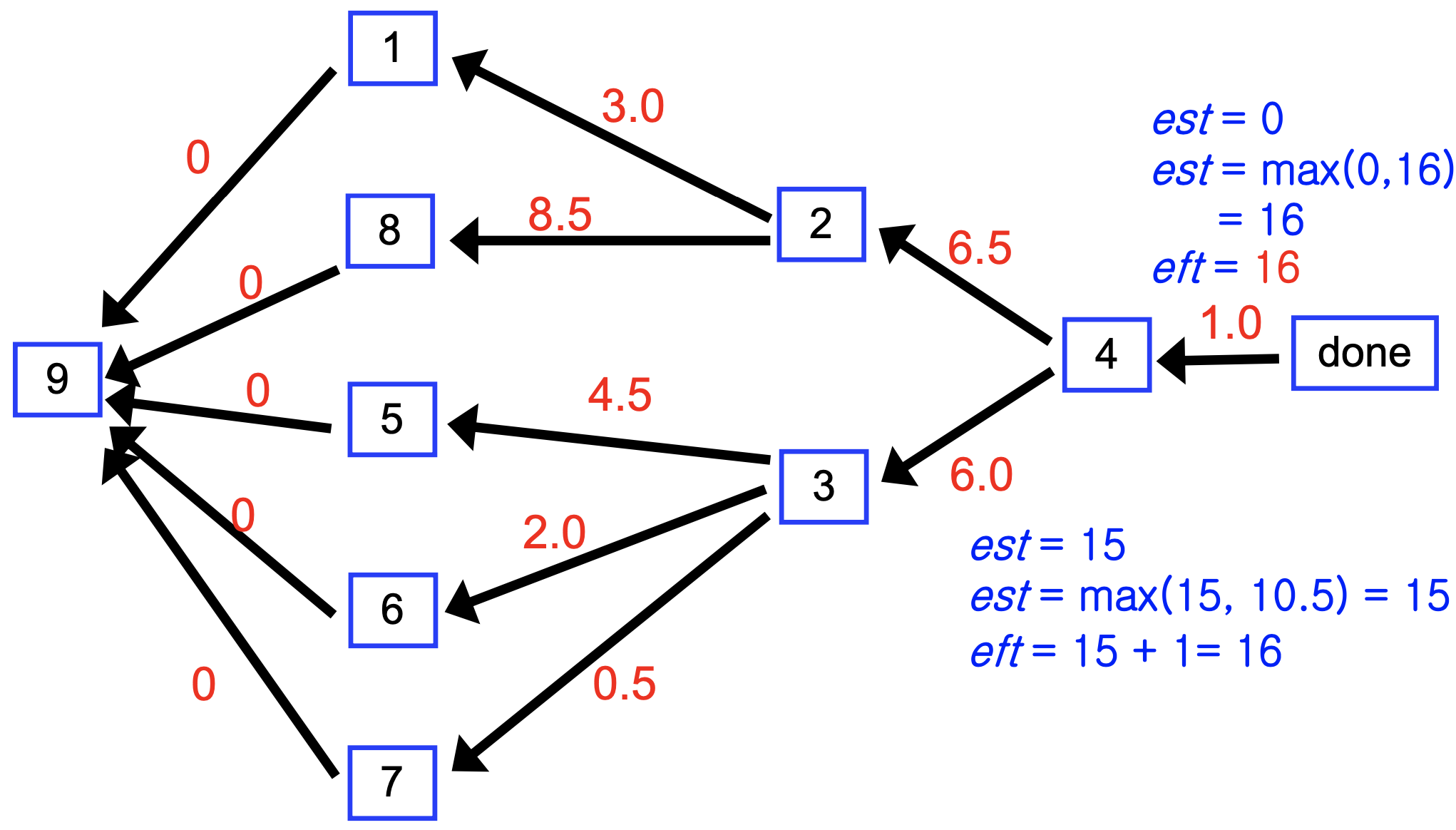
Modified DAG
- Add a special task to the project, called done, with duration 0; it can be task number n+1
- Every regular task that is not a dependency of any task (i.e., potential final task) is made a dependency of done
- The project DAG has a weighted edge vw whenever v depends on w (reverse the direction), and the weight of this edge is the duration of w
Algorithm
- DFS on project DAG.When backtracking edge vw
if eft[w] > est[v]
	est[v] = eft[w]
Crit_Dep[v] = w // w로 부터오는 길이 critical path- At postorder processing time, insert
eft[v] = est[v] + duration[v]
Example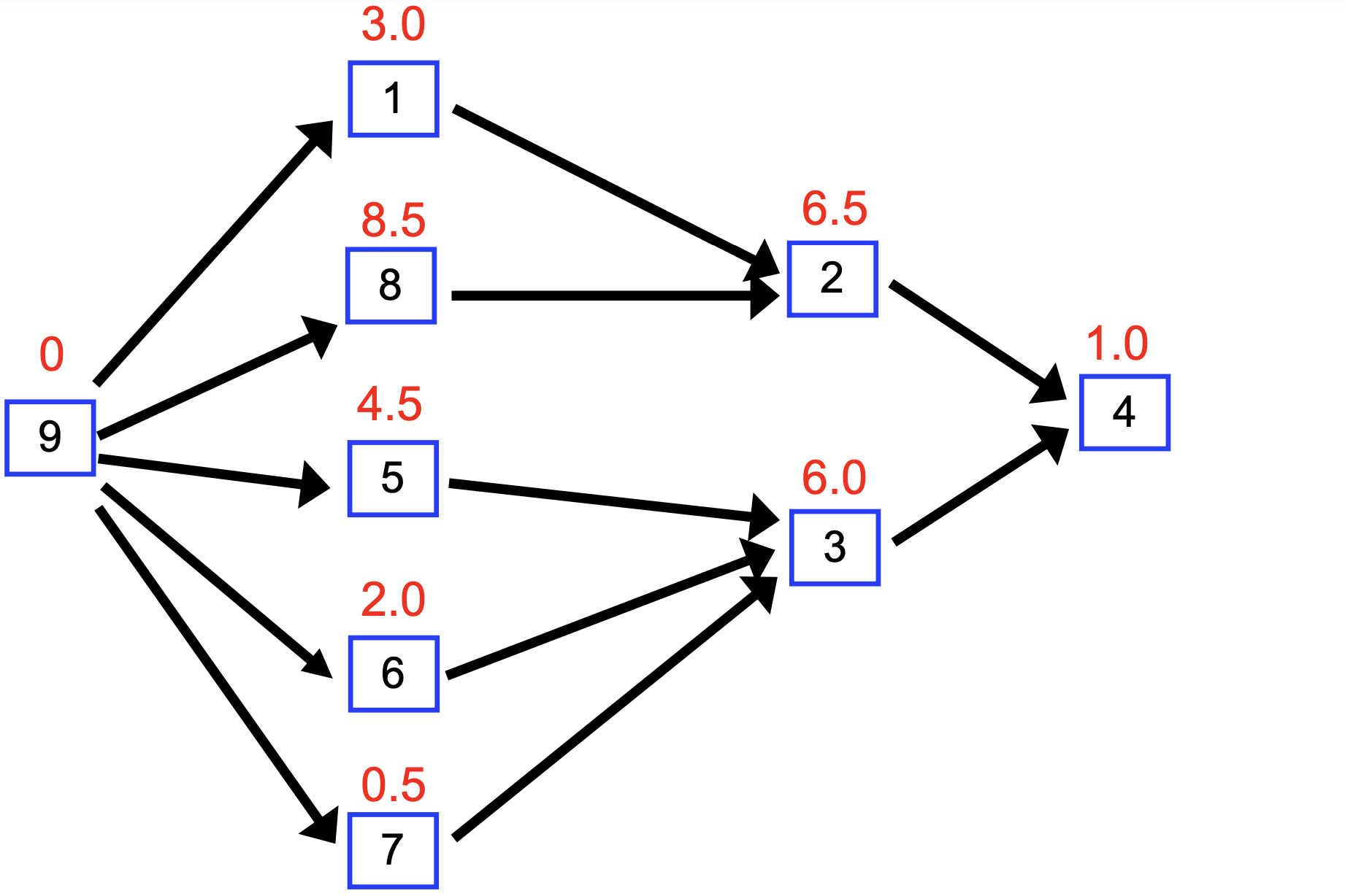
Exercise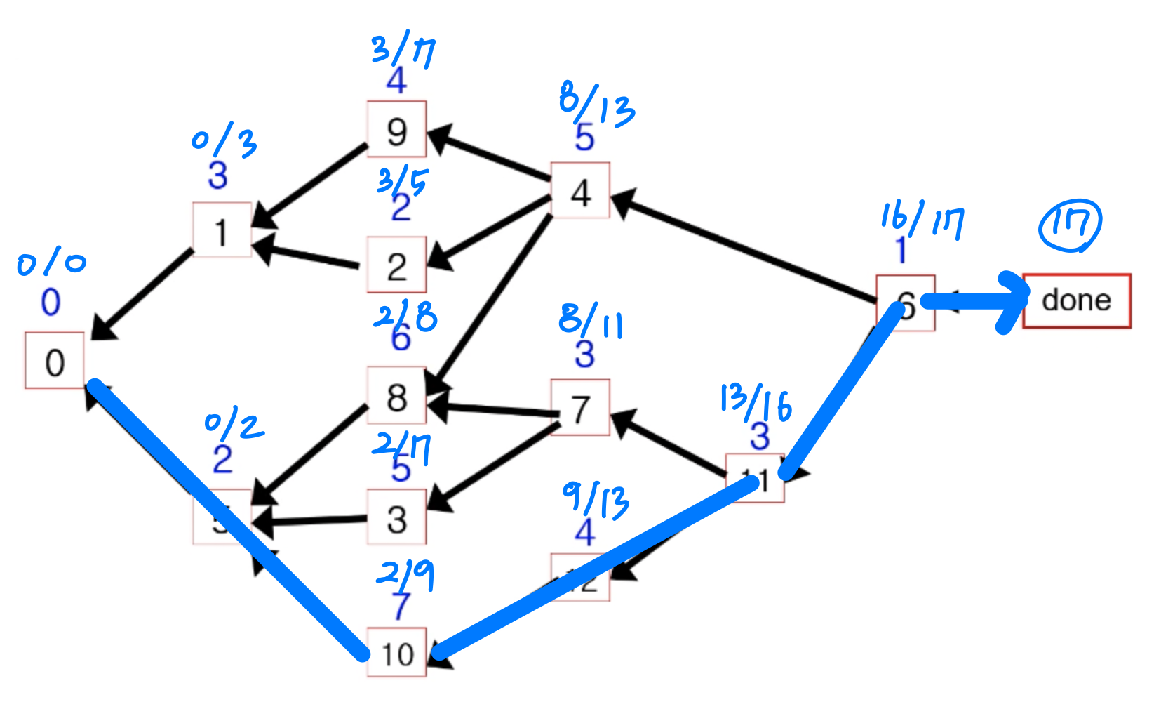
5) Bi-connected Components (AP)
- Problem:
- If any one vertex (and the edges incident upon it) are removed from a connected graph, is the remaining subgraph still connected?
- Biconnected graph: ➡️ 하나의 node가 없어지더라도 connected
- If it remains connected after removal of any one vertex and the edges that are incident upon that vertex
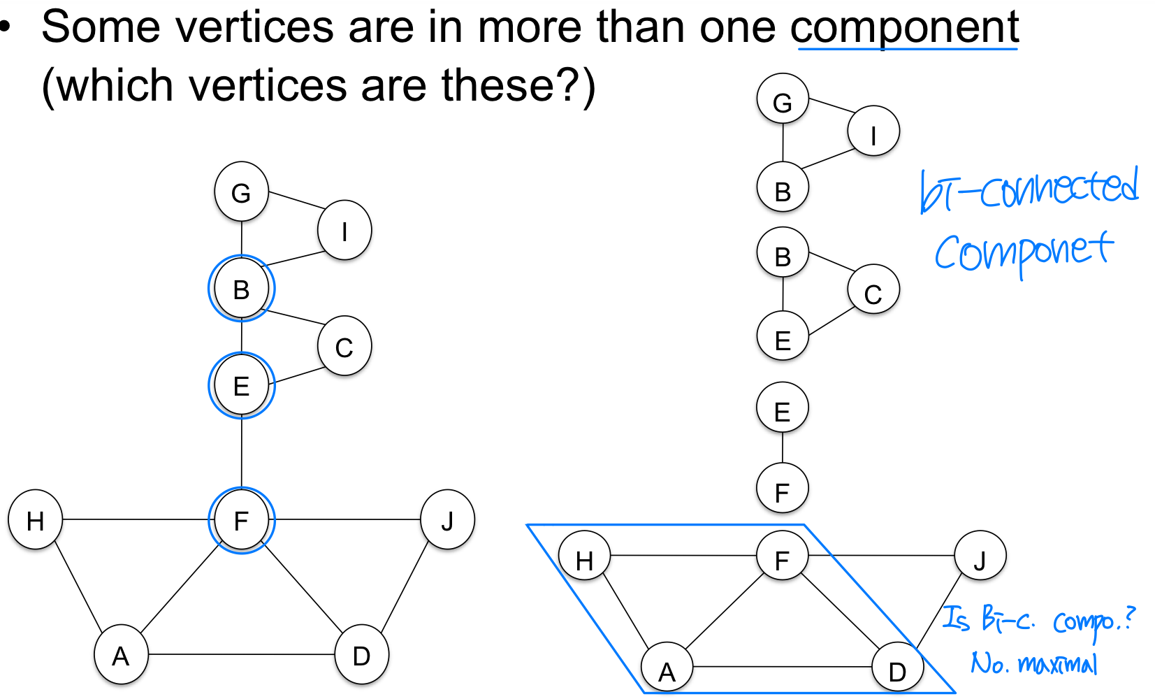
- Biconnected component:
- A biconnected component of a undirected graph is a maximal biconnected subgraph, that is, a binconnected subgraph not contained in any larger binconnected subgraph.
- Articulation point:
- If there are distinct vertices w and x (distinct from v also) such that v is in every path from w to x (에 항상 포함)
Articulation Point
- Fact
- Every edge is either tree edge or back edge
- Leaf cannot be articulation point
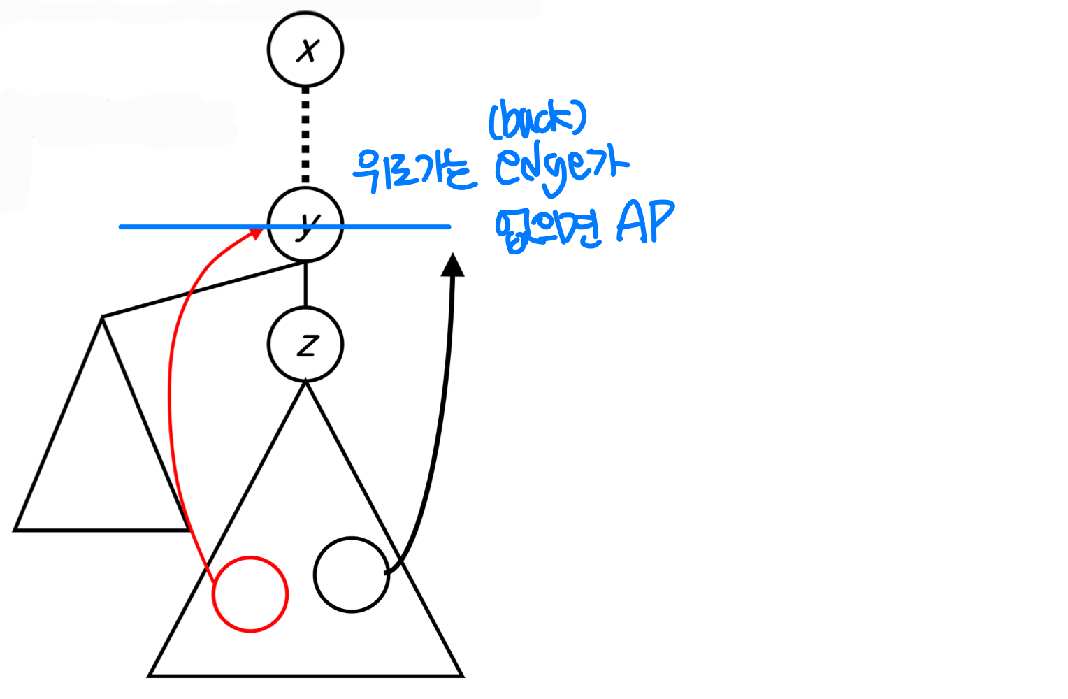
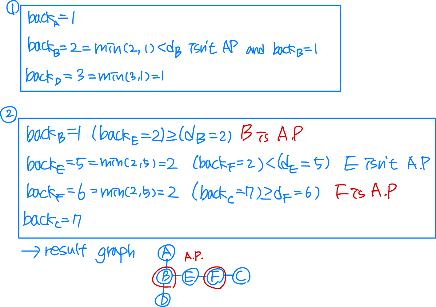
- ⭐️ When backing up from z to y, if there is no back edge from any vertex in the subtree rooted at z to proper ancestor of y(y위로), y is articulation point
- Call DFS on the graph. We store ‘back’
- For all v < y, check back edge vw.
a. back is initialized to d[v]
b. When encounteded with back edge vw
back = min (, d(w))
c. When backtracking from v to u,
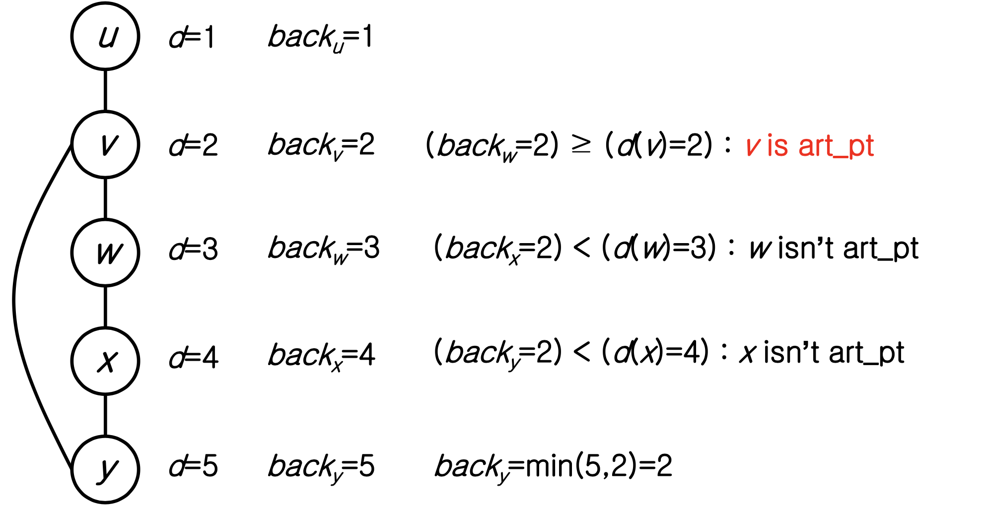
back = min(back, back) - When backing up form z to y,
if all vertices ≤ z, back ≥ d(y). : y is art_pt. else back < d(y). : y isn’t art_pt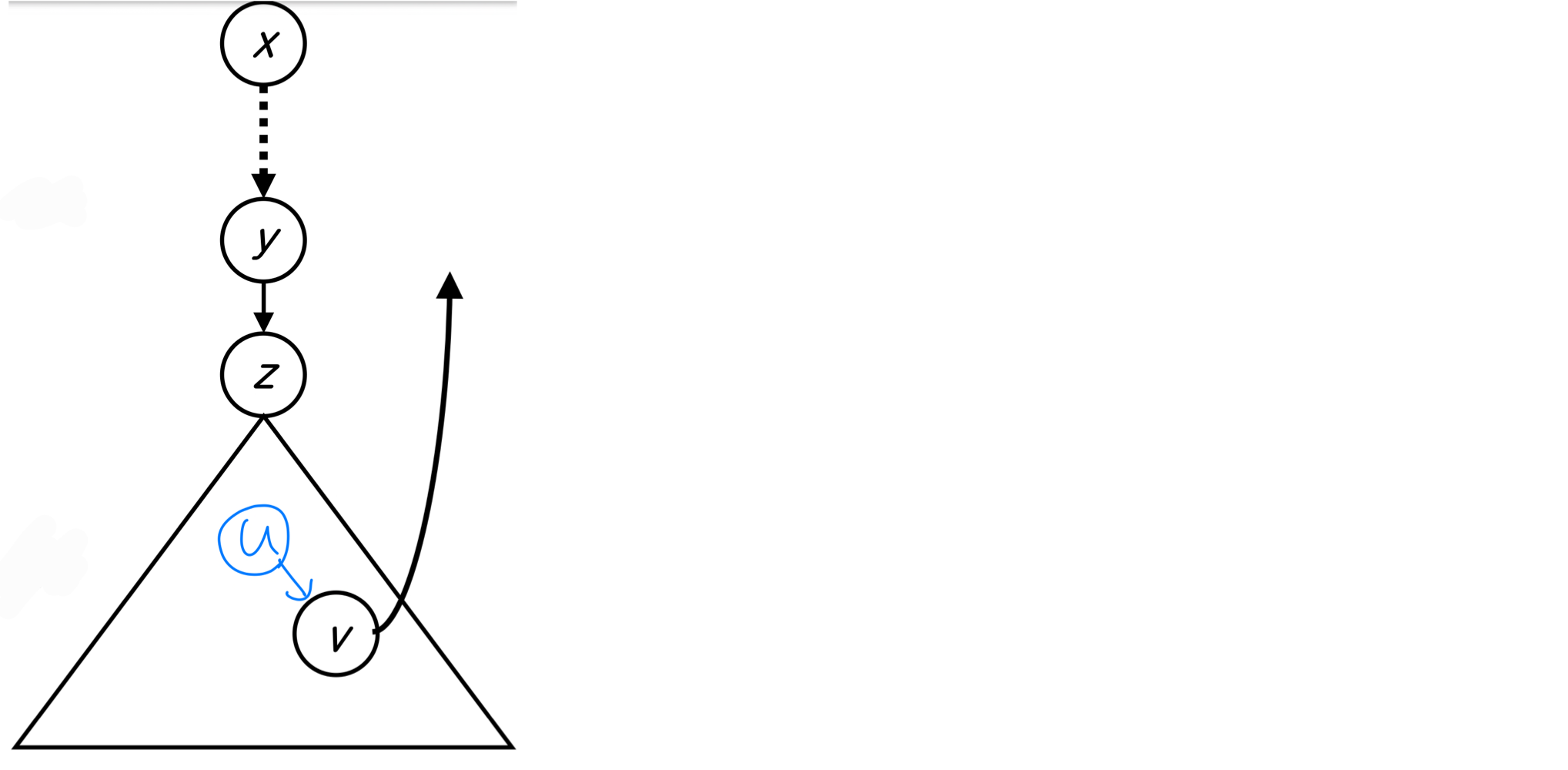
Example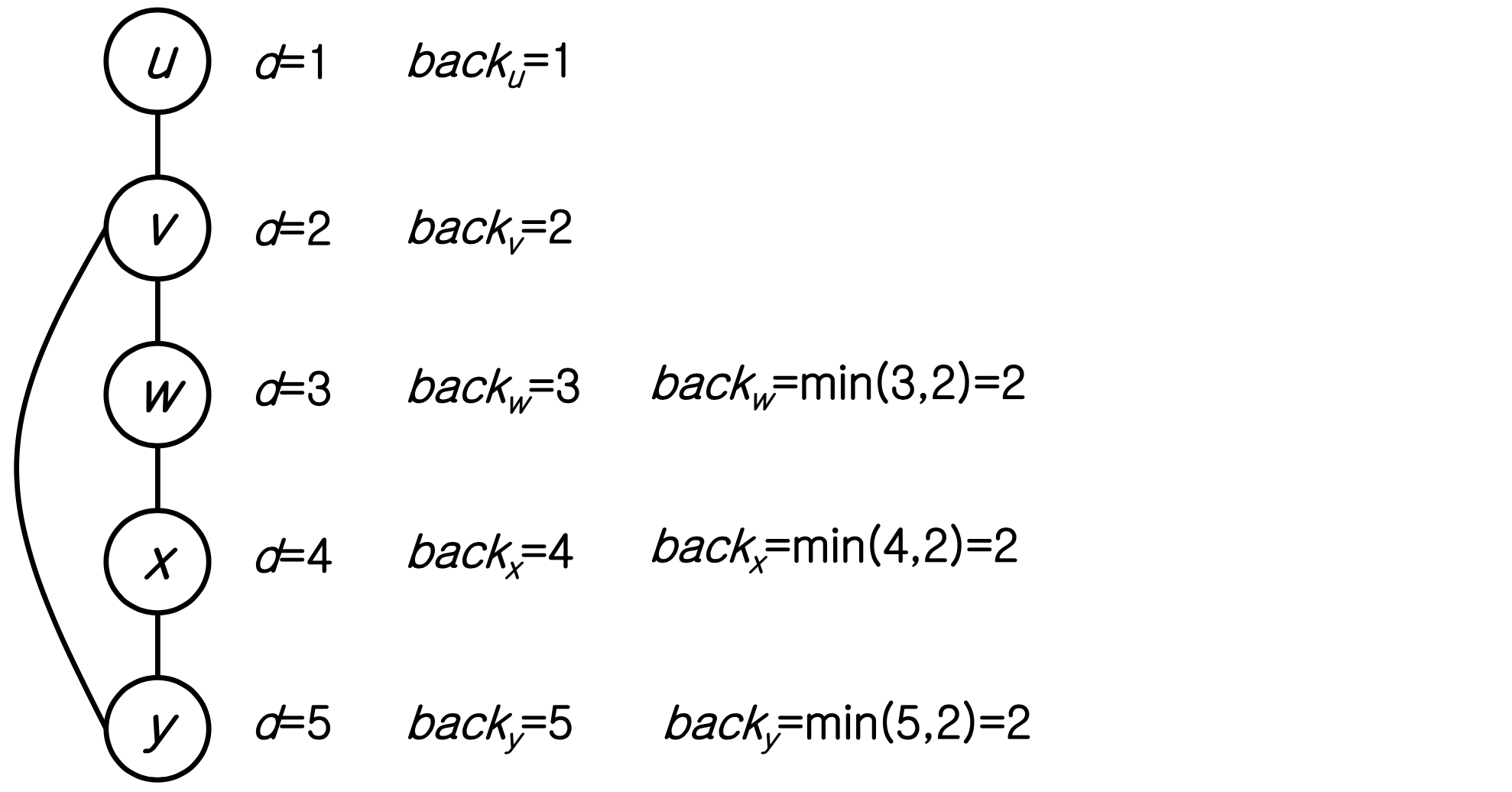
- Biconnected components and AP
- A ⭐️ root of DFS tree is an articulation point iff it has at least two children ➡️ child 하나면 AP X
- A non-root vertex u is an articulation point iff it has at least one child
- A ⭐️ root of DFS tree is an articulation point iff it has at least two children ➡️ child 하나면 AP X
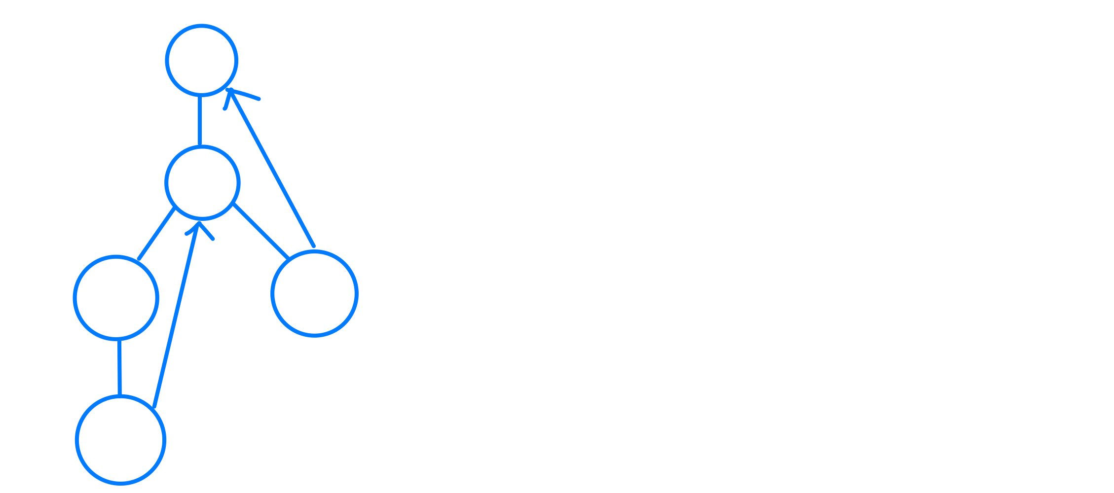
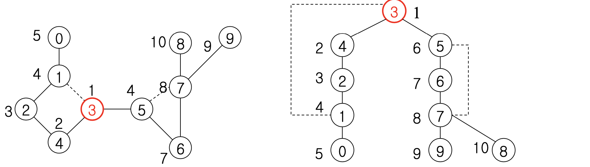
Exercise
Identify articulation point on the following graph. Assume the vertices are in alphabetical order in the Adj array and that each adjacency list is in alphabetical order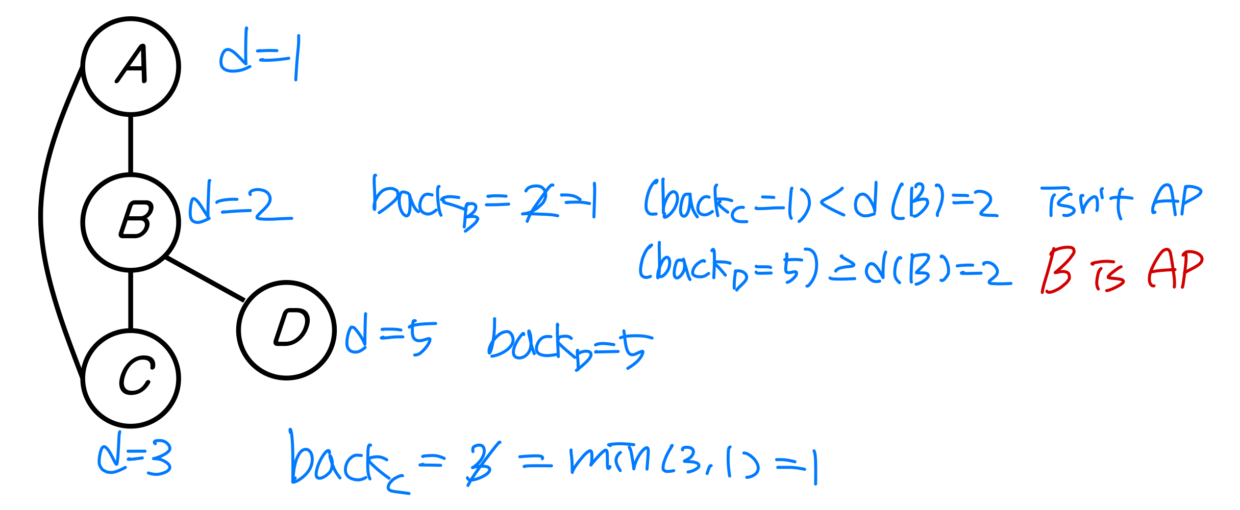
🖥️ Exercise in class
1. Draw the adj matrix, and adj list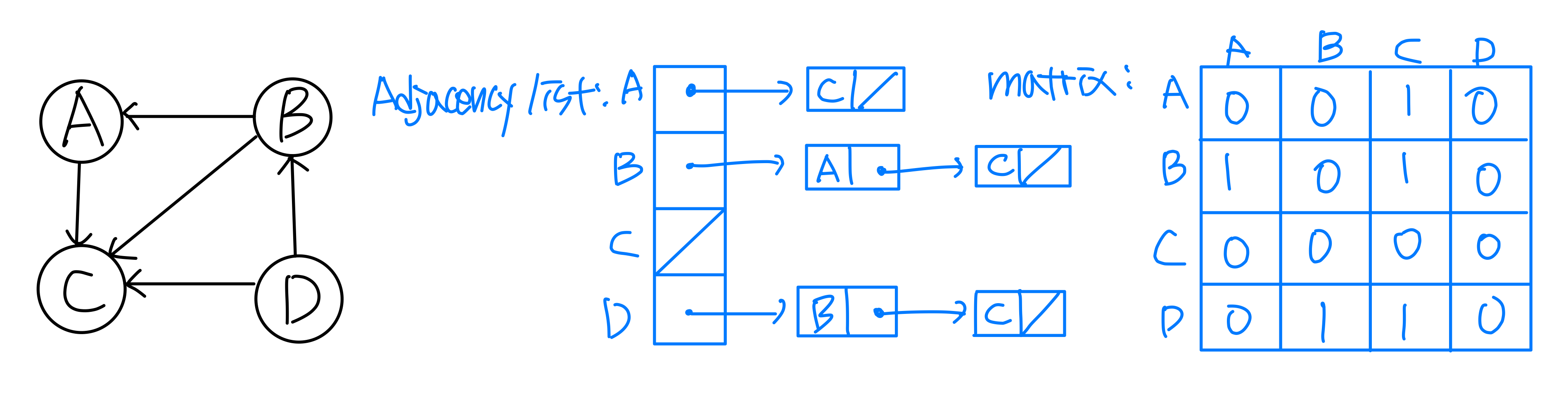
➡️ Space complexity : matrix - (V), list - (V+E)
2. BFS
Show the d and values that result from running BFS, use vertex 3 as the source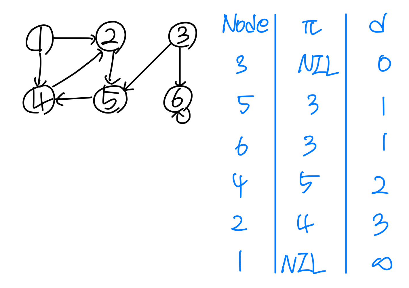
3. BFS running time
1) Adjacency list : (V+E)
2) matrix, modify the algorithm to handle this form of input : (V)
DFS? same (V+E)
➡️ 그렇다면 asymtotically faster algorith이 있을까? NO.
DFS : Type of edges
Assume the vertices are in alphabetic order in Adj array and each adj list in alphabetic order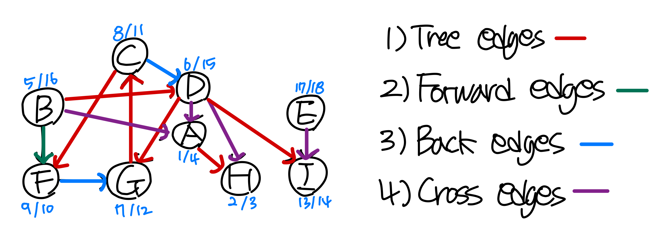
4. How do we associate finish time and vertices?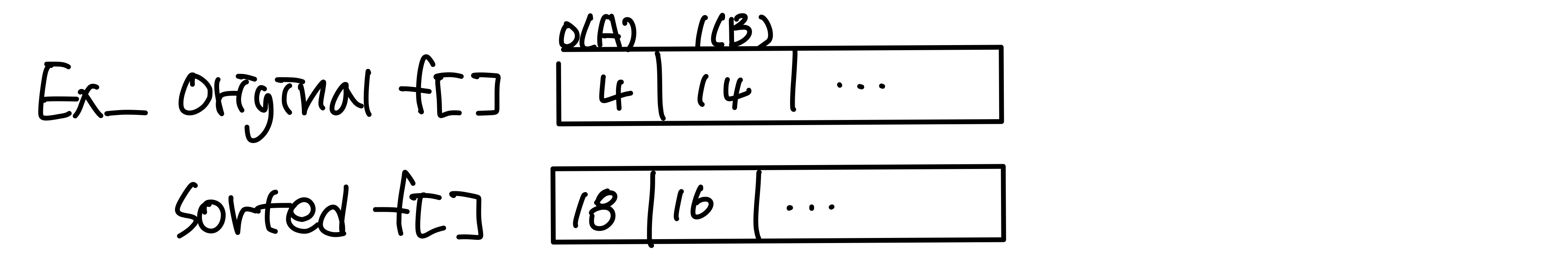
A. structure or extra array
5. SCC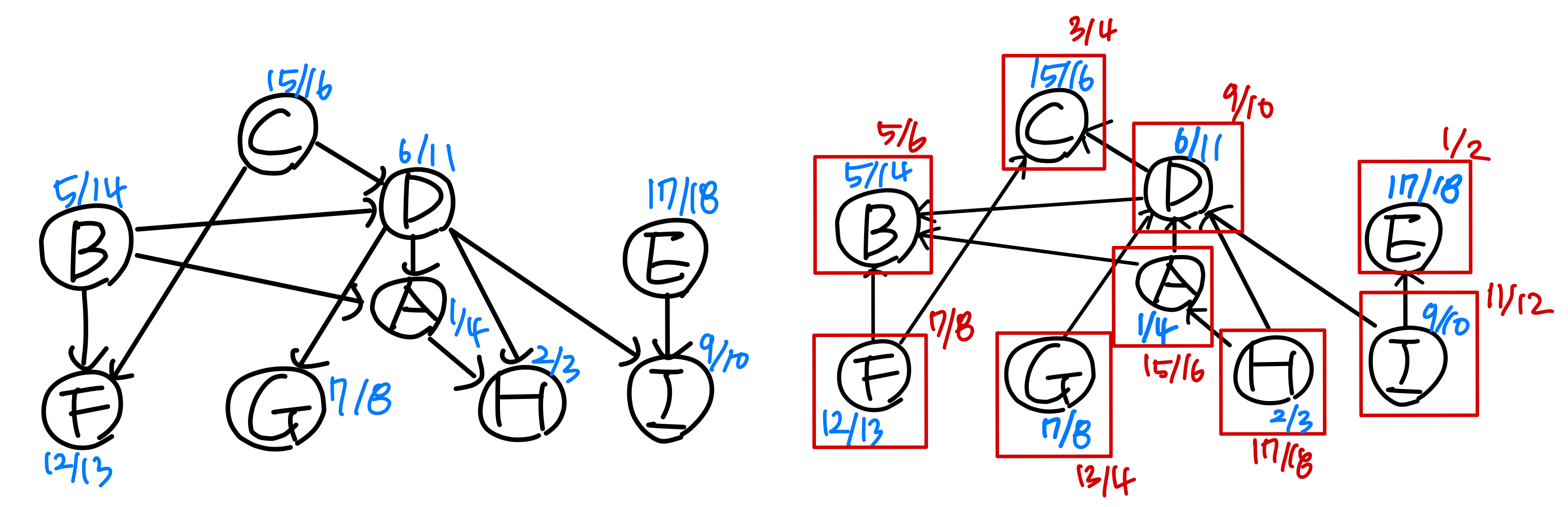
6. Critical Pass
Determine 'est' and 'eft' of each node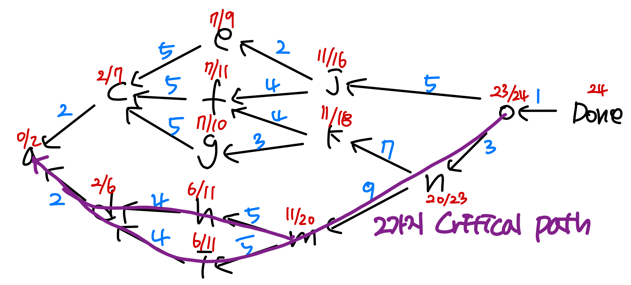
7. AP
when node B가 AP가 될 때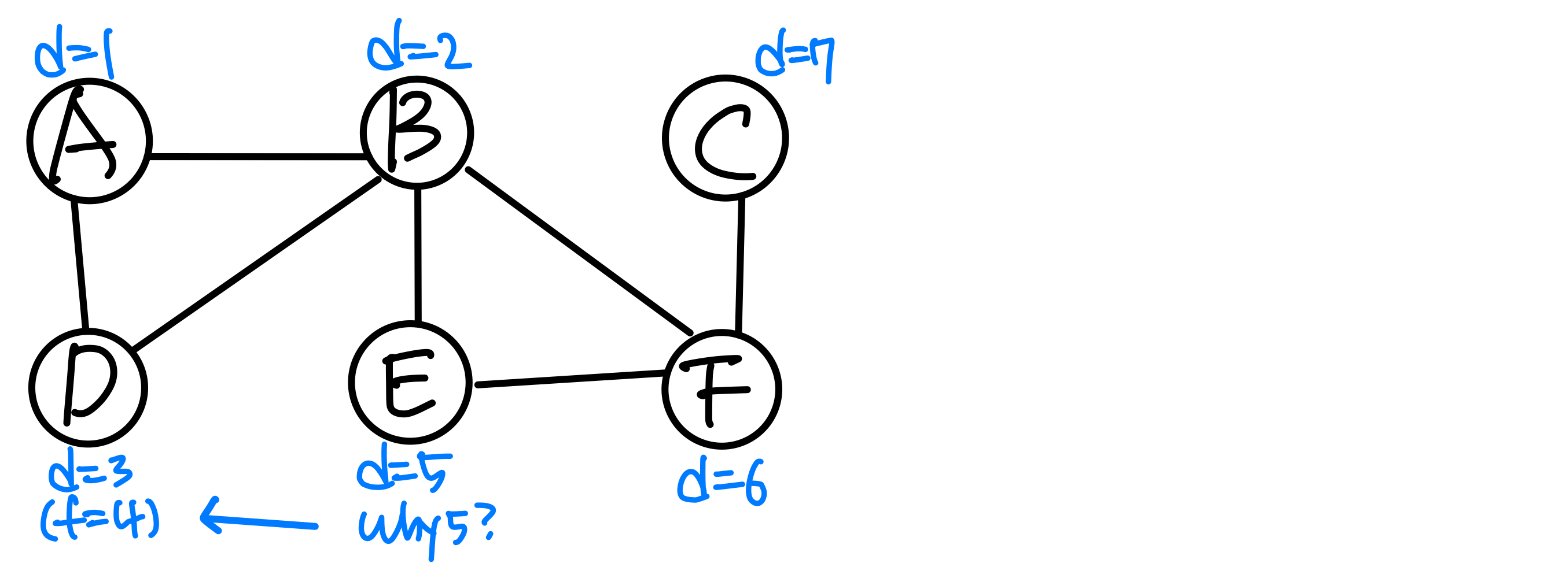
HGU 전산전자공학부 용환기 교수님의 23-1 알고리듬 분석 수업을 듣고 작성한 포스트이며, 첨부한 모든 사진은 교수님 수업 PPT의 사진 원본에 필기를 한 수정본입니다.