[ Algorithm ] 13. Sorting in Linear-Time

Sorting So Far

• Insertion sort: → O(n$^2$)
  selection Θ(n$^2$), bubble Θ(n$^2$)
  • Easy to code
  • Fast on small inputs (less than ~50 elements)
  • Fast on nearly-sorted inputs
  • Θ(n$^2$) worstcase
  • Θ(n$^2$) average (equally-likely inputs) case
• Merge sort: → Stable
  • Divide-and-conquer:
    • Split array in half
    • Recursively sort subarrays • Linear-time merge step
  • Θ(n lg n)
  • Doesn’t sort in place
• Heap sort: → not a stable
  • Uses the very useful heap data structure
    • Complete binary tree
    • Heap property: parent key > children’s keys
  • Θ(n lg n) worst case
  • Sorts in place
• Quick sort:
  • Divide-and-conquer: → not a stable, not sort in place
    • Partition array into two subarrays, the recursive calling.
    • All of first subarray < all of second subarray
    • No merge step needed!
  • Θ(n lg n) average case
  • Fast in practice
  • Θ(n$^2$) worst case

How Fast Can We Sort?

• We will provide a lower bound, then beat it
  • How do you suppose we’ll beat it?
• First, an observation: all of the sorting algorithms so far are comparison sorts
  • The only operation used to gain ordering information about a sequence is the pairwise comparison of two elements
  • Theorem: all comparison sorts are $\Omega$(n lg n)
    • Is this the best we can do?

Decision tree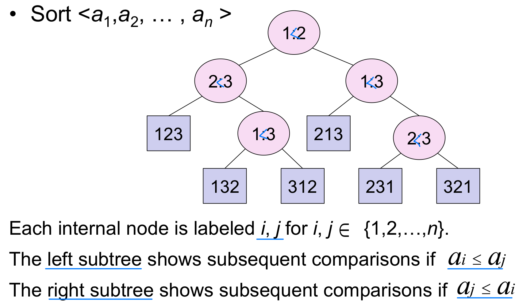

Decision tree Example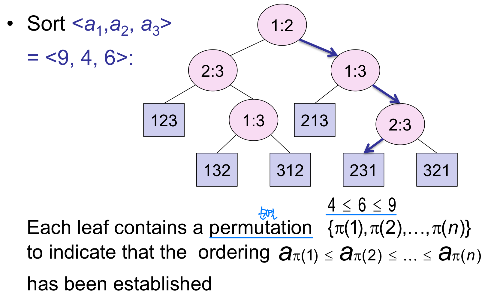

Decision tree model

• A decision tree can model the execution of any comparison sort:
  • One tree for each input size n
  • View the algorithm as slitting whenever it compares two elements.
  • The tree contains the comparisons along all possible instruction traces.
  • The running time of the algorithm = the length of the path taken.
  • Worst-case running time = height of tree

Lower bound for decision tree sorting

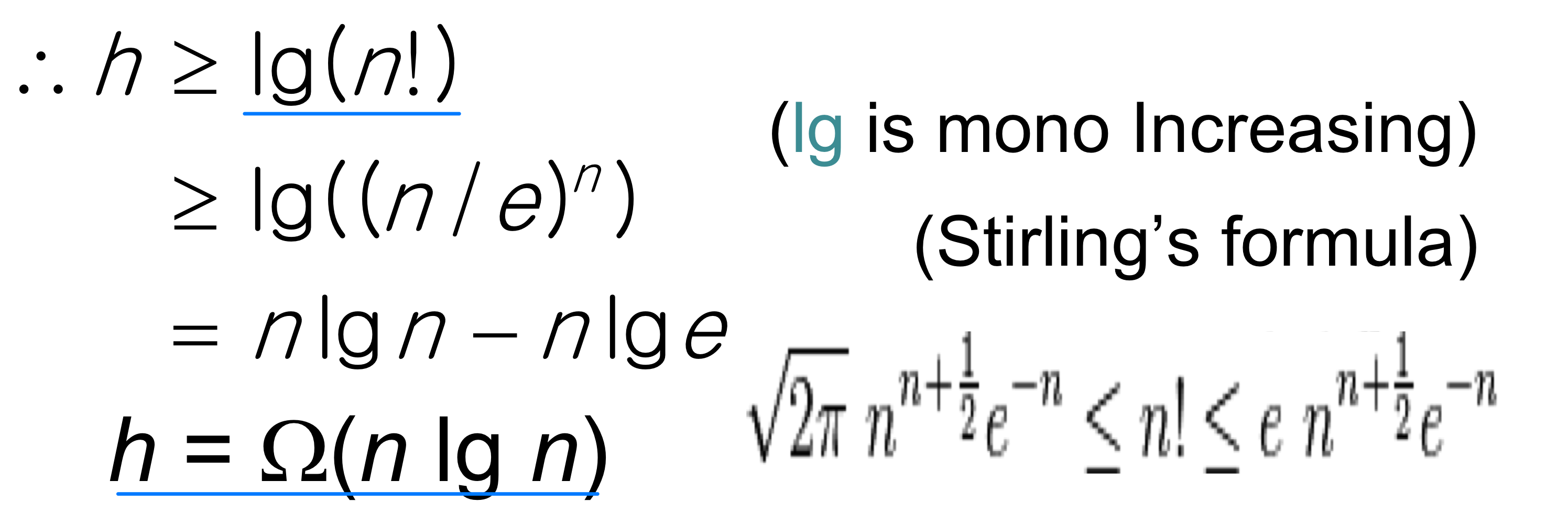
• Theorem. Any decision tree that can sort n elements must have height $\Omega$(n lgn)
• Proof. The tree must contain ≥ n! leaves, since there are n! possible permutations. A height-h binary tree has ≤ 2h leaves. Thus, n! ≤ 2h

Lower Bound For Comparison Sort

• Thus the time to sort n elements with comparison sort is $\Omega$(n lg n)
• Corollary: Heapsort and Mergesort are asymptotically optimal comparison sorts
• But the name of this lecture is “Sorting in linear time”!
  • How can we do better than $\Omega$(n lg n)?

---

Counting-sort

• Counting-Sort does not use comparisons
• Counting-Sort uses counting to sort
• We can sort an input array in Θ(n) time!!
• Constraints
  • Each of the n input elements should be an INTEGER
  • Each of the n input elements should be in the range 0 to k, for some integer k.
  • It should be possible to represent that k = O(n)

Sorting In Linear Time

• Input / Output:
  • Input: A[1..n], where A[j] $\in$ {1, 2, 3, ..., k}
  • Output: B[1..n], sorted (notice: does not sort in place)
  • Also: Array C[0..k] for auxiliary storage is needed.
• BasicIdea
  • The basic idea of counting sort is to determine, for each input element x, the number of elements less than x
  • This information can be used to place element x directly into its position in the output array

Pesudo-code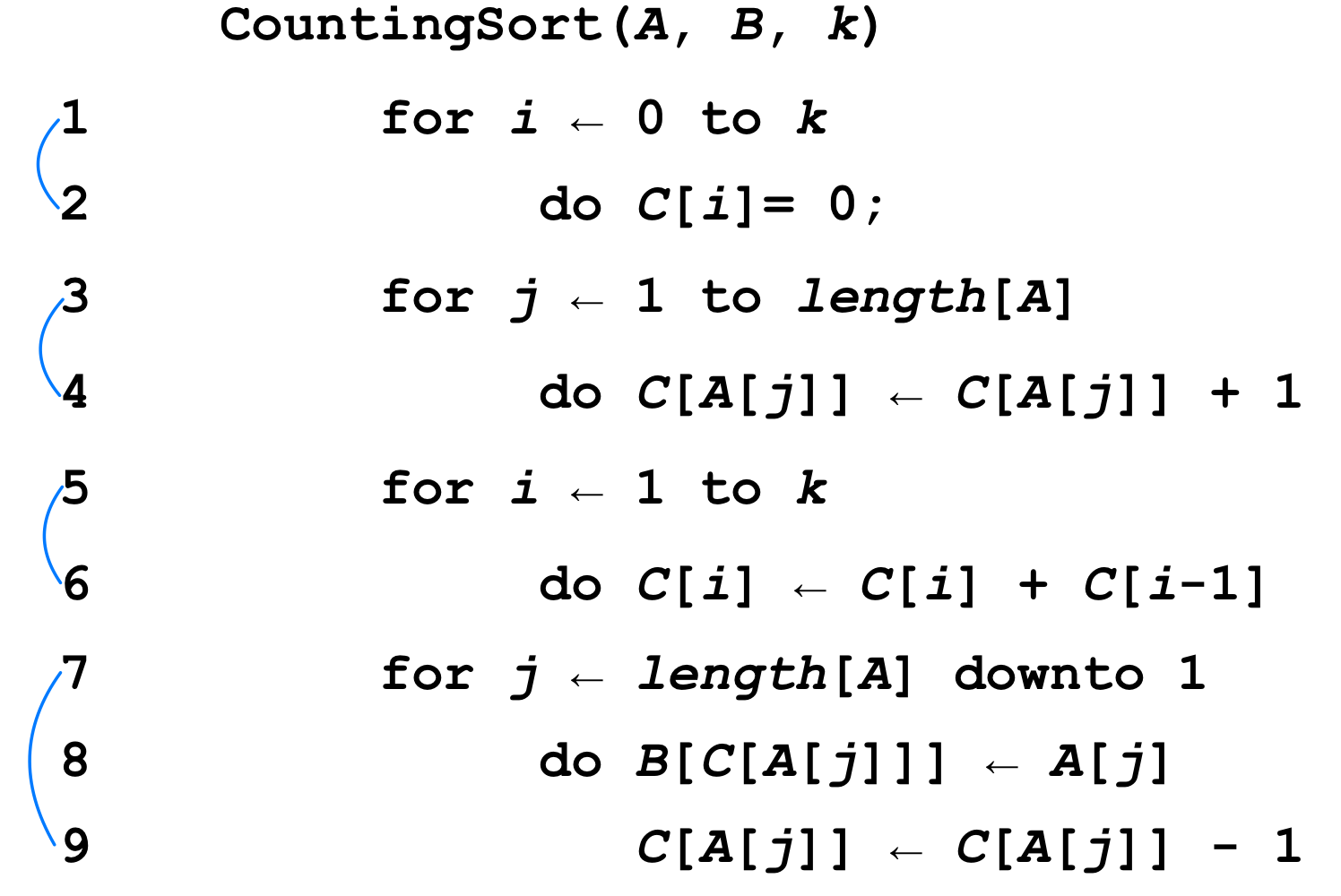

Line 1-2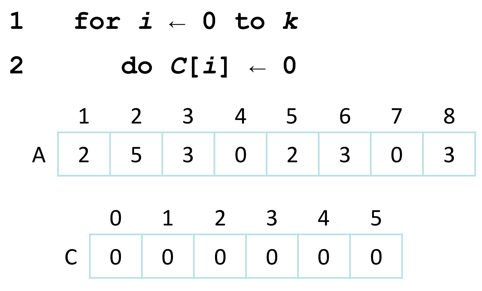

Line 3-4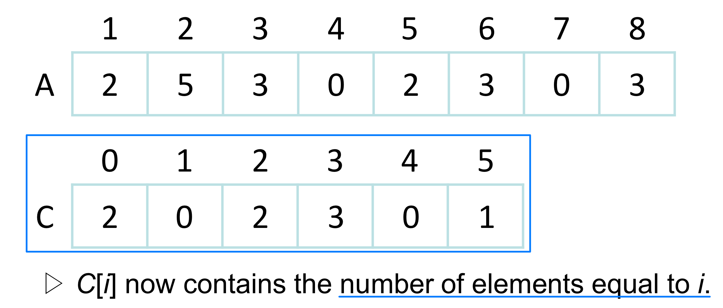

Line 5-6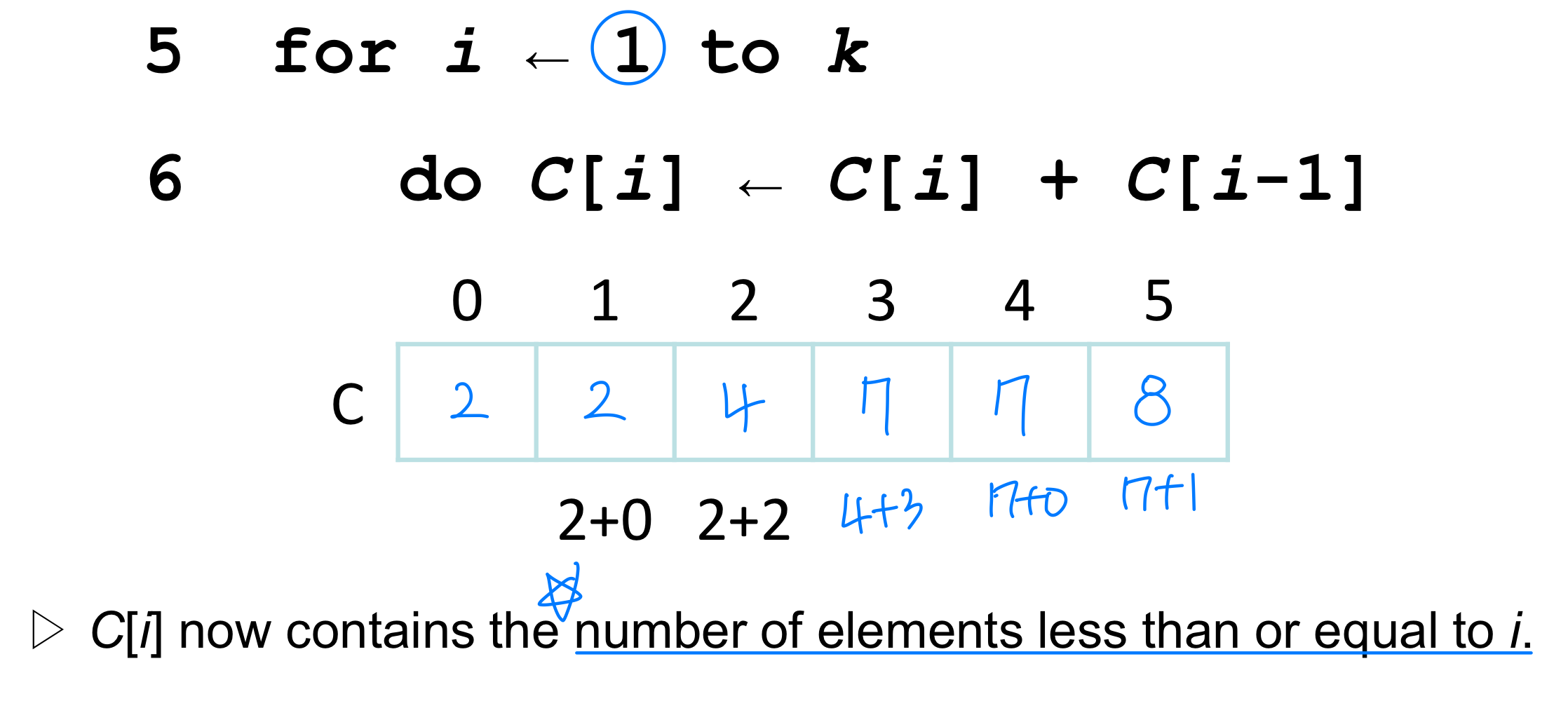

Line 7-9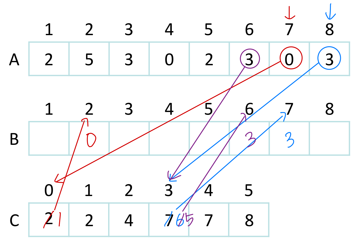→ For stable sort, from length[A] to 1

Analysis of counting sort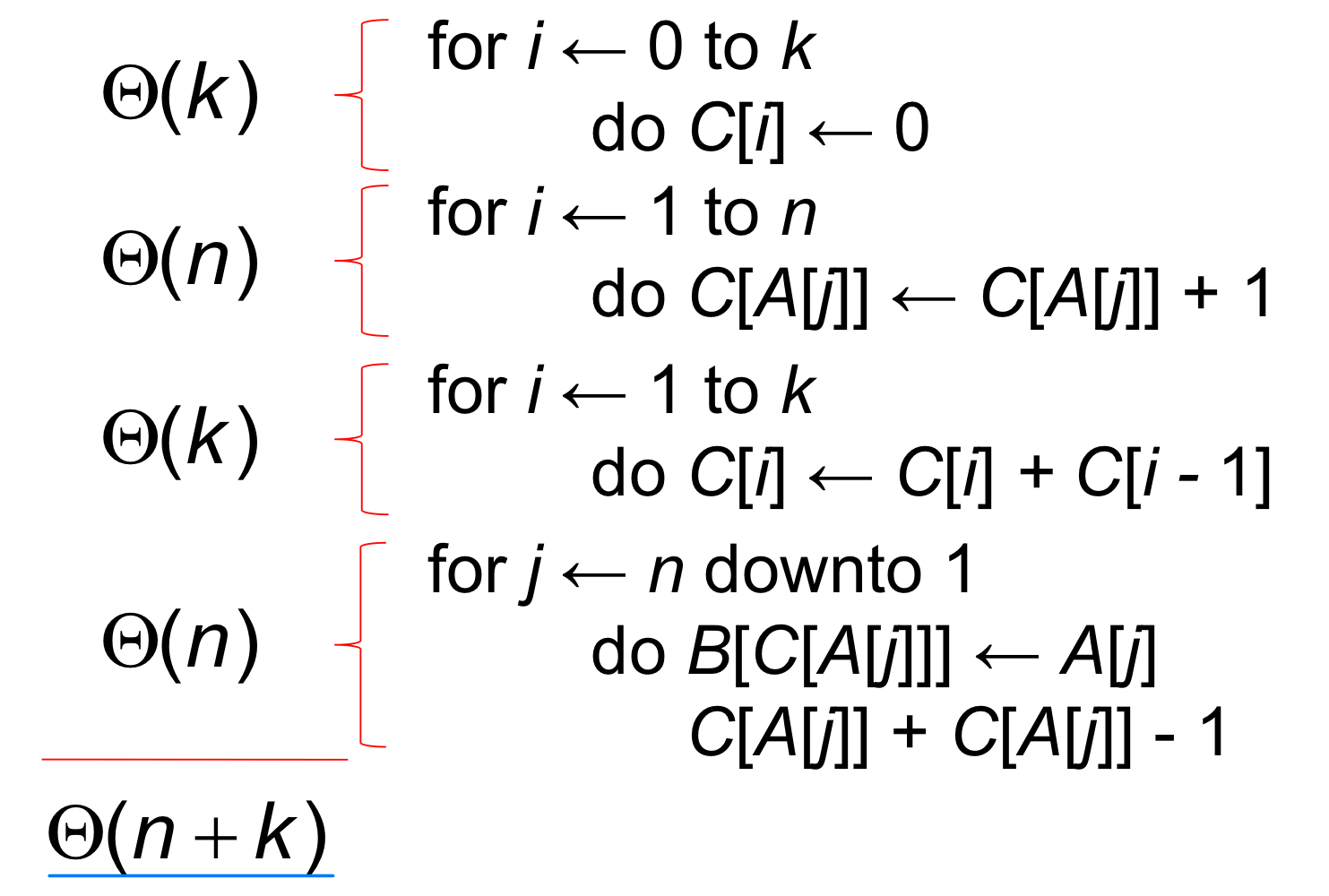

Running time

• If ⭐️ k = O(n), then counting sort takes Ө(n) time.
  • But, sorting takes Ω(n lg n) time!
  • Where’s the fallacy?
• Answer:
  • Comparison sorting takes Ω(n lg n) time.
  • Counting sort is not a comparison sort
  • In fact, not a single comparison between elements occurs!
    
    
• Cool! Why don’t we always use counting sort?
• Because it depends on range k of elements
• Could we use counting sort to sort 32 bit integers? Why or why not?
• Answer: no, k too large (2$^{32}$ = 4,294,967,296) → k = O(n)이라고하기 힘듬

Stable sorting

Counting sort is a stable sort: it preserves the input order among equal elements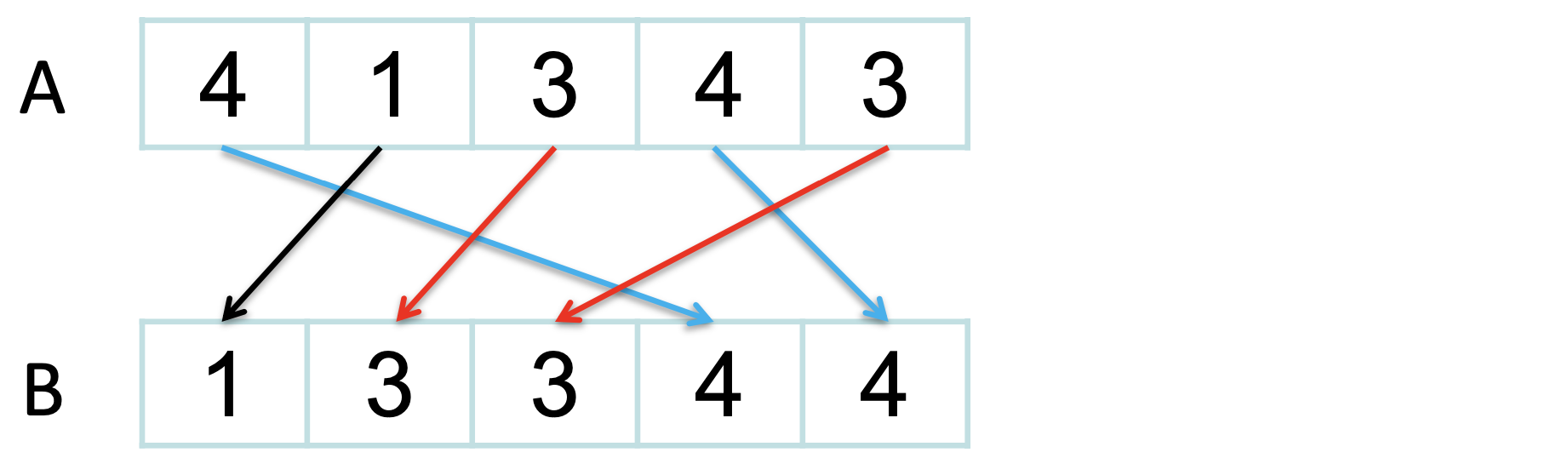Exercise: What other sorts have this property?
→ Normally, the property of stability is important only when satellite data are carried around with the element being sorted. Counting-Sort is often used as a subroutine in radix sort.

---

Radix Sort

Number of keys : not one, but several keys... say d keys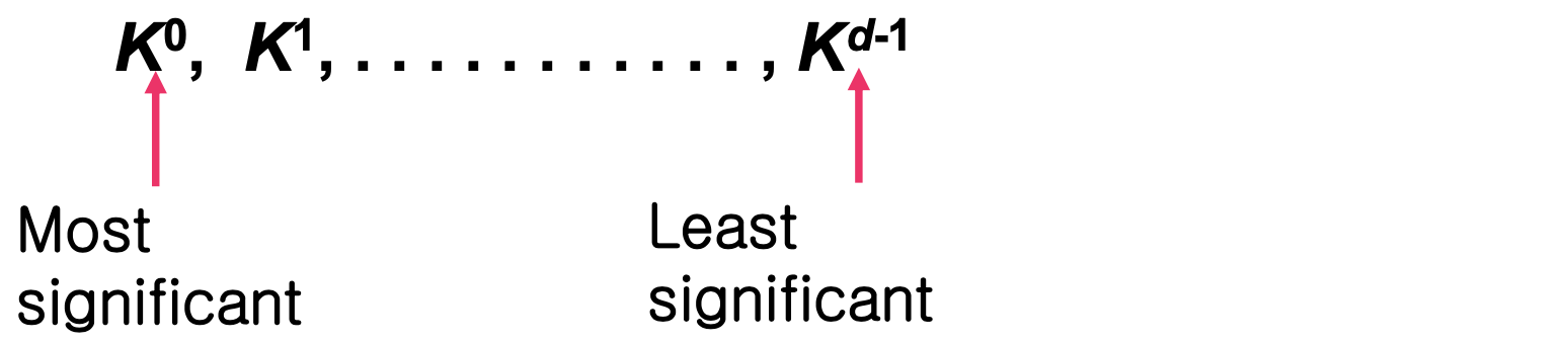Ex) Sorting students by class, math. score, height
Ex) Sorting deck of cards
Two keys - (1) suit : clover < diamond < heart < spade
                    (2) face value : 2 < 3 < 4 < . . . . . . < J < Q < K < A After sorting,
2C, 3C, ... KC, AC, 2D, 3D, .......... < KS < AS(Ace Spade)

[1] MSD : Most Significant Digit
Step 1 : Sort by suit
Step 2 : Sort by face value
[2] LSD : Least Significant Digit
Step 1 : Sort by face
Step 2 : Sort by suit

• Intuitively, you might sort on the most significant digit, then the second msd, etc.
• Problem: lots of intermediate piles of cards to keep track of
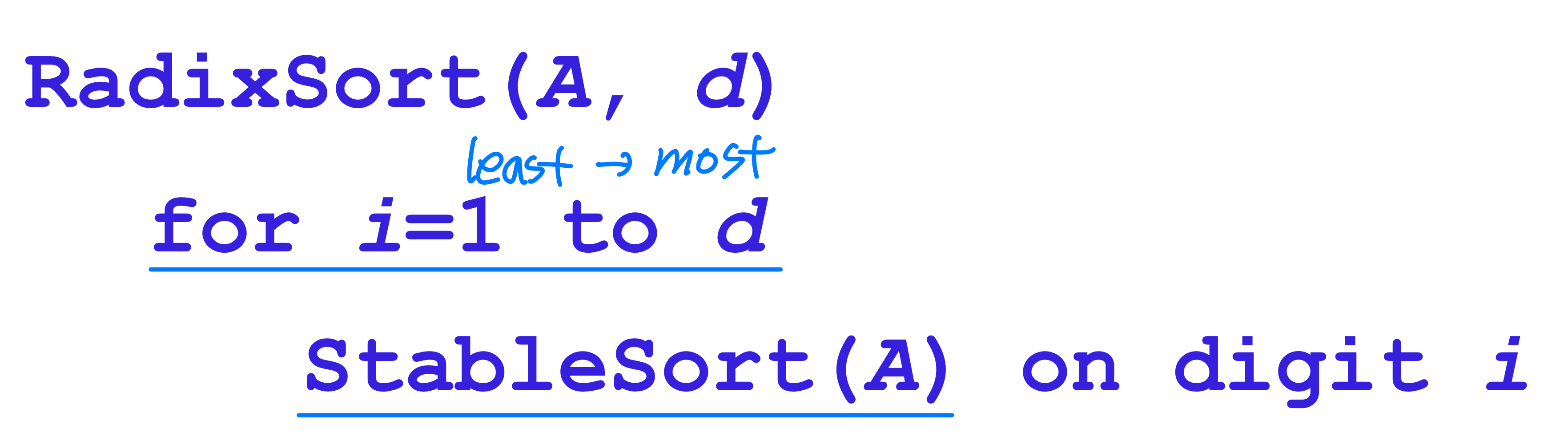
• Key idea: sort the ⭐️ least significant digit first

Example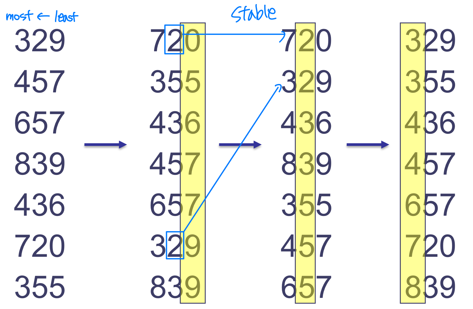

More radix sort

• Can we prove it will work? ( with LSD )
• Sketch of an inductive argument (induction on the
  number of passes):
  • Assume lower-order digits { j: j<i } are sorted
  • Show that sorting next digit i leaves array correctly sorted
    • If two digits at position i are different, ordering numbers by that digit is correct (lower-order digits irrelevant)
    • If they are the same, numbers are already sorted on the lower-order digits. Since we use a stable sort, the numbers stay in the right order
      
      
• What sort will we use to sort on digits?
• Counting sort is obvious choice:
  • Sort n numbers on digits that range from 1..k
  • Time: Θ(n+k)
• Each pass over n numbers with d digits takes time Θ(n+k), so total time Θ(dn+dk)
  • When d is constant and k=O(n), it takes Θ(n) time
    
    
• In general, radix sort based on counting sort is
  • Fast
  • Asymptotically fast (i.e., Θ(n))
  • Simple to code
  • A good choice

---

Bucket Sort

• Bucketsort
  • Assumption: input is n reals from [0, 1]
  • Basic idea:
    • Create n lists ( buckets(hash) ) to divide interval [0,1] into subintervals of size 1/n
    • Add each input element to appropriate bucket and sort buckets with insertion sort
• Uniform(일정한) input distribution → Θ(1) bucket size
  • Therefore the expected total time is Θ(n)
• The idea as discussed in hash table

Worst-case

→ 한쪽으로 치우쳤을 때 그 address에 있는 element를 다시 sort

• Lemma: In the worst case, Bucket Sort takes O(n$^2$) time
• Using Merge Sort, we can get this down to Θ(n lg n).
• But Insertion Sort is simpler

Average-case

• Lemma: Given that the input sequence is drawn uniformly at random from [0,1), the expected size of a bucket is Θ(1)
• Lemma: Given that the input sequence is drawn uniformly at random from [0,1), the average-case running time of Bucket Sort is Θ(n)

---

Summary

• Every comparison-based sorting algorithm has to take Ω(n lg n) time
• Merge Sort, Heap Sort, and Quick Sort are comparison- based and take Θ(n lg n) time. Hence, they are optimal
• Other sorting algorithms can be faster by exploiting assumptions made about the input
• Counting Sort and Radix Sort take linear time for integers in a bounded range
• Bucket Sort takes linear average-case time for uniformly distributed real numbers

---

Exercise in Class

1. sort in place and stable sort

Sort in place : If only a constant number of elements of input are ever stored outside the array
Ex) insertion, heap, quick

Stable sort : Elements with the same key appear in the ouptut array in the same order as they do in the input array
Ex) insertion sort, merge sort, counting sort

2. Counting sort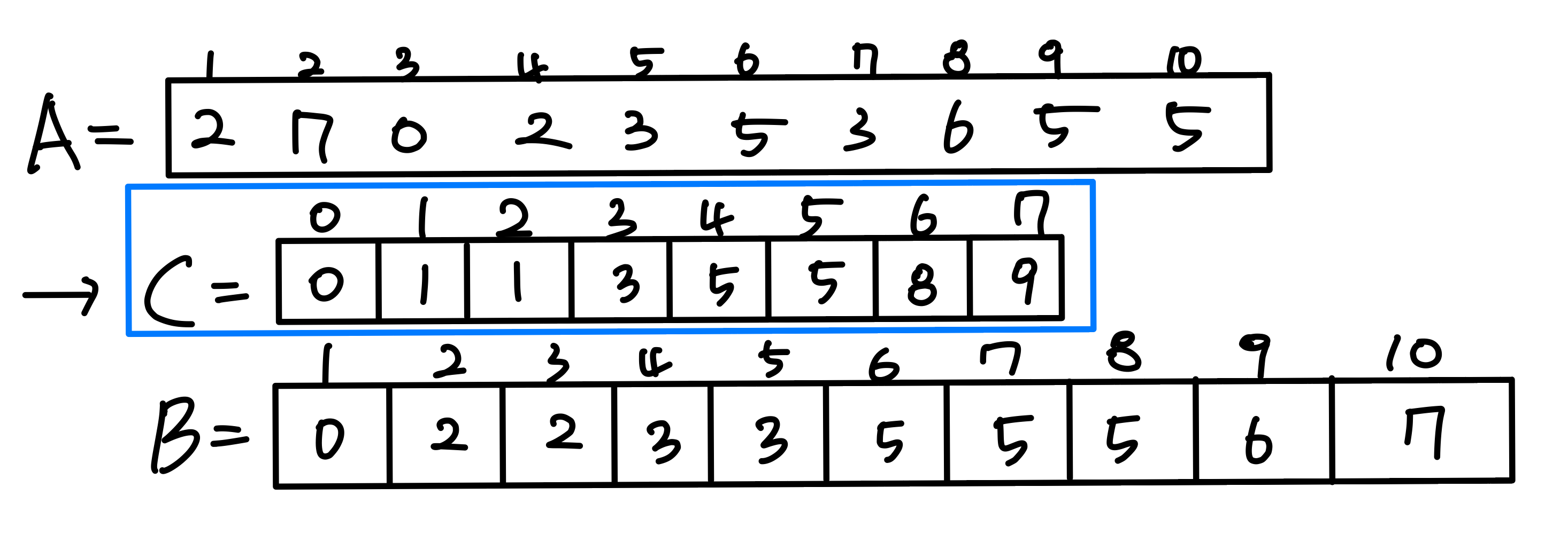

HGU 전산전자공학부 용환기 교수님의 23-1 알고리듬 분석 수업을 듣고 작성한 포스트이며, 첨부한 모든 사진은 교수님 수업 PPT의 사진 원본에 필기를 한 수정본입니다.