컴퓨터 비전을 위한 전이학습(Transfer Learning)

전이학습(Transfer Learning)
: 어떤 목적을 이루기 위해 학습된 모델을 다른 작업에 이용하는 것
- 이미 학습된 pre-trained 모델을 가져오고 마지막 레이어만 새로 학습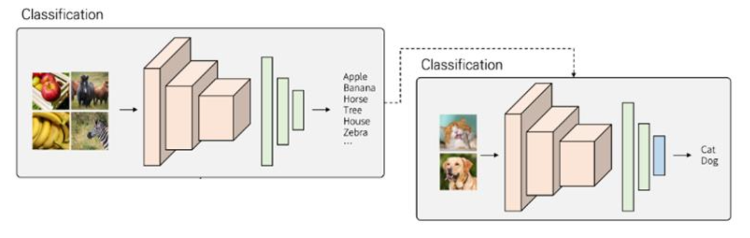- ImageNet, ResNet, ...
- 학습이 빠르게 수행된다
- overfitting을 예방할 수 있다

이러한 전이학습 시나리오의 중요한 2가지는 다음과 같다:

• Condition
  • pretrained 데이터와 새로운 데이터가 비슷한 형태를 가지는 경우
  • 새로운 데이터보다 pretrained 데이터의 양이 더 많은 경우
• fine-tuning
  • transfer learning에서 사용되는 기법 중 하나
  • 사전 학습된 모델을 새로운 문제에 적용하기 위해 일부 가중치를 조절 하는 학습 과정

# License: BSD
# Author: Sasank Chilamkurthy

from __future__ import print_function, division

import torch
import torch.nn as nn
import torch.optim as optim
from torch.optim import lr_scheduler
import torch.backends.cudnn as cudnn
import numpy as np
import torchvision
from torchvision import datasets, models, transforms
import matplotlib.pyplot as plt
import time
import os
import copy

cudnn.benchmark = True
plt.ion()   # 대화형 모드

Load Data

# 학습을 위해 데이터 증가(augmentation) 및 일반화(normalization)
# 검증을 위한 일반화
data_transforms = {
    'train': transforms.Compose([
        transforms.RandomResizedCrop(224),
        transforms.RandomHorizontalFlip(),
        transforms.ToTensor(),
        transforms.Normalize([0.485, 0.456, 0.406], [0.229, 0.224, 0.225])
    ]),
    'val': transforms.Compose([
        transforms.Resize(256),
        transforms.CenterCrop(224),
        transforms.ToTensor(),
        transforms.Normalize([0.485, 0.456, 0.406], [0.229, 0.224, 0.225])
    ]),
}

data_dir = 'data/hymenoptera_data'
image_datasets = {x: datasets.ImageFolder(os.path.join(data_dir, x),
                                          data_transforms[x])
                  for x in ['train', 'val']}
dataloaders = {x: torch.utils.data.DataLoader(image_datasets[x], batch_size=4,
                                             shuffle=True, num_workers=4)
              for x in ['train', 'val']}
dataset_sizes = {x: len(image_datasets[x]) for x in ['train', 'val']}
class_names = image_datasets['train'].classes

device = torch.device("cuda:0" if torch.cuda.is_available() else "cpu")

• data augmentation과 normalization을 위한 전처리 과정
• datasets.ImageFolder – 학 습과 검증용 데이터셋 불러오 기
• torch.utils.data.DataLoader – 데이터를 학습에 활용할 수 있도록 batch로 나눔

일부 이미지 시각화하기

def imshow(inp, title=None):
    """tensor를 입력받아 일반적인 이미지로 보여줍니다."""
    inp = inp.numpy().transpose((1, 2, 0))
    mean = np.array([0.485, 0.456, 0.406])
    std = np.array([0.229, 0.224, 0.225])
    inp = std * inp + mean
    inp = np.clip(inp, 0, 1)
    plt.imshow(inp)
    if title is not None:
        plt.title(title)
    plt.pause(0.001)  # 갱신이 될 때까지 잠시 기다립니다.


# 학습 데이터의 배치를 얻습니다.
inputs, classes = next(iter(dataloaders['train']))

# 배치로부터 격자 형태의 이미지를 만듭니다.
out = torchvision.utils.make_grid(inputs)

imshow(out, title=[class_names[x] for x in classes])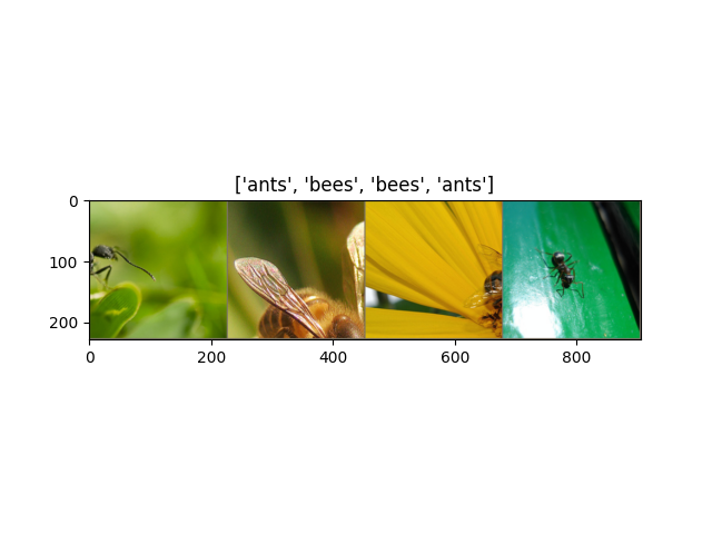

데이터 증가를 이해하기 위해 일부 학습용 이미지를 시각화

Training model

def train_model(model, criterion, optimizer, scheduler, num_epochs=25):
    since = time.time()

    best_model_wts = copy.deepcopy(model.state_dict())
    best_acc = 0.0

    for epoch in range(num_epochs):
        print(f'Epoch {epoch}/{num_epochs - 1}')
        print('-' * 10)

        # 각 에폭(epoch)은 학습 단계와 검증 단계를 갖습니다.
        for phase in ['train', 'val']:
            if phase == 'train':
                model.train()  # 모델을 학습 모드로 설정
            else:
                model.eval()   # 모델을 평가 모드로 설정

            running_loss = 0.0
            running_corrects = 0

            # 데이터를 반복
            for inputs, labels in dataloaders[phase]:
                inputs = inputs.to(device)
                labels = labels.to(device)

                # 매개변수 경사도를 0으로 설정
                optimizer.zero_grad()

                # 순전파
                # 학습 시에만 연산 기록을 추적
                with torch.set_grad_enabled(phase == 'train'):
                    outputs = model(inputs)
                    _, preds = torch.max(outputs, 1)
                    loss = criterion(outputs, labels)

                    # 학습 단계인 경우 역전파 + 최적화
                    if phase == 'train':
                        loss.backward()
                        optimizer.step()

                # 통계
                running_loss += loss.item() * inputs.size(0)
                running_corrects += torch.sum(preds == labels.data)
            if phase == 'train':
                scheduler.step()

            epoch_loss = running_loss / dataset_sizes[phase]
            epoch_acc = running_corrects.double() / dataset_sizes[phase]

            print(f'{phase} Loss: {epoch_loss:.4f} Acc: {epoch_acc:.4f}')

            # 모델을 깊은 복사(deep copy)함
            if phase == 'val' and epoch_acc > best_acc:
                best_acc = epoch_acc
                best_model_wts = copy.deepcopy(model.state_dict())

        print()

    time_elapsed = time.time() - since
    print(f'Training complete in {time_elapsed // 60:.0f}m {time_elapsed % 60:.0f}s')
    print(f'Best val Acc: {best_acc:4f}')

    # 가장 나은 모델 가중치를 불러옴
    model.load_state_dict(best_model_wts)
    return model

• scheduling the learning rate
• saving the best model
• train_model 함수는 딥러닝 model의 학습과 검증을 수행하는 함수

scheduler 매개변수는 torch.optim.lr_scheduler 의 LR 스케쥴러 객체(Object)이다.

모델 예측값 시각화하기

def visualize_model(model, num_images=6):
    was_training = model.training
    model.eval()
    images_so_far = 0
    fig = plt.figure()

    with torch.no_grad():
        for i, (inputs, labels) in enumerate(dataloaders['val']):
            inputs = inputs.to(device)
            labels = labels.to(device)

            outputs = model(inputs)
            _, preds = torch.max(outputs, 1)

            for j in range(inputs.size()[0]):
                images_so_far += 1
                ax = plt.subplot(num_images//2, 2, images_so_far)
                ax.axis('off')
                ax.set_title(f'predicted: {class_names[preds[j]]}')
                imshow(inputs.cpu().data[j])

                if images_so_far == num_images:
                    model.train(mode=was_training)
                    return
        model.train(mode=was_training)

일부 이미지에 대한 예측값을 보여주는 일반화된 함수

합성곱 신경망 미세조정 ( Finetuning )

• learning rate scheduler는 학습 도중 학습률을 동적으로 조정하여 학 습 과정을 최적화 하는 기법 중 하나
• 초기에는 높은 학습률로 시작하여 빠르게 수렴하게 하고, 학습이 진 행됨에 따라 학습률을 조금씩 낮추어 더 정교하게 최적점을 찾도록 하는 방식
• 학습이 진행될수록 학습률이 감소하여 더 세밀하게 최적화

model_ft = models.resnet18(weights='IMAGENET1K_V1')
num_ftrs = model_ft.fc.in_features
# 여기서 각 출력 샘플의 크기는 2로 설정합니다.
# 또는, ``nn.Linear(num_ftrs, len (class_names))`` 로 일반화할 수 있습니다.
model_ft.fc = nn.Linear(num_ftrs, 2)

model_ft = model_ft.to(device)

criterion = nn.CrossEntropyLoss()

# 모든 매개변수들이 최적화되었는지 관찰
optimizer_ft = optim.SGD(model_ft.parameters(), lr=0.001, momentum=0.9)

# 7 에폭마다 0.1씩 학습률 감소
exp_lr_scheduler = lr_scheduler.StepLR(optimizer_ft, step_size=7, gamma=0.1)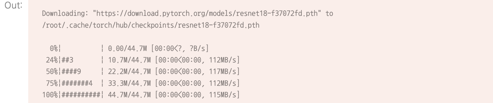

미리 학습한 모델을 불러온 후 마지막의 완전히 연결된 계층을 초기화

학습 및 평가하기

CPU에서는 15-25분 가량, GPU에서는 1분도 이내의 시간이 걸린다.

model_ft = train_model(model_ft, criterion, optimizer_ft, exp_lr_scheduler,
                       num_epochs=25)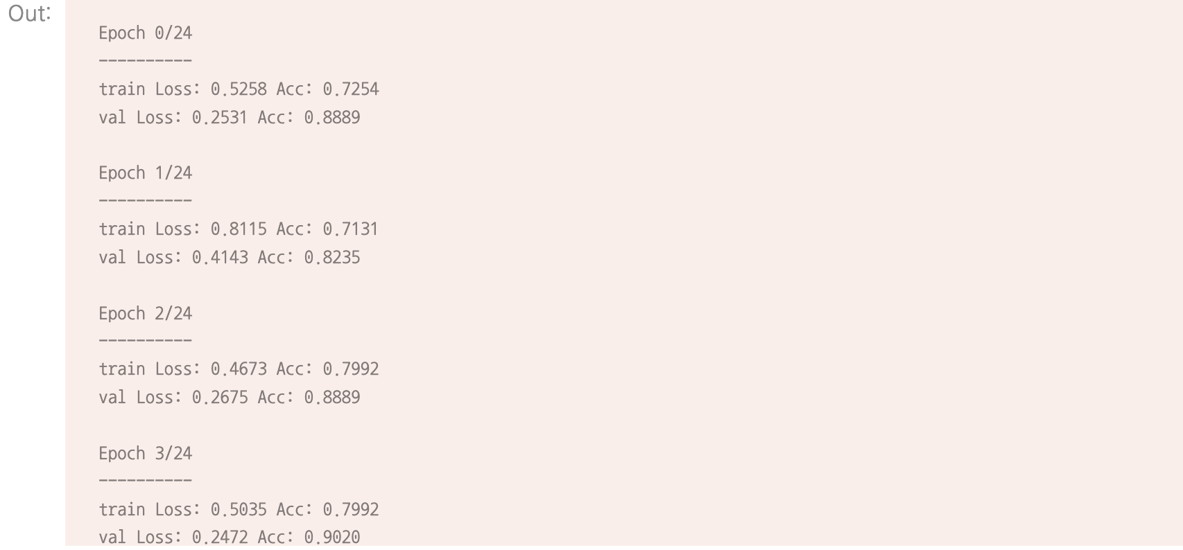

visualize_model(model_ft)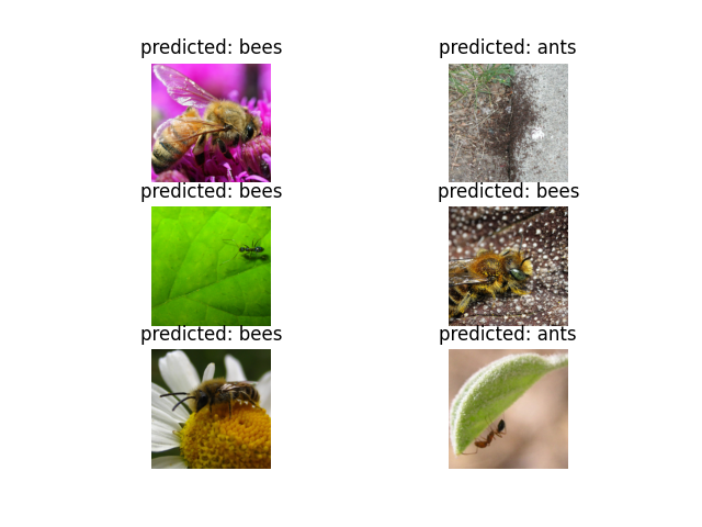

고정된 특징 추출기로써의 합성곱 신경망

pretrained 데이터들의 매개변수 고정, 가중치 그대로 사용

model_conv = torchvision.models.resnet18(weights='IMAGENET1K_V1')
for param in model_conv.parameters():
    param.requires_grad = False

# 새로 생성된 모듈의 매개변수는 기본값이 requires_grad=True 임
num_ftrs = model_conv.fc.in_features
model_conv.fc = nn.Linear(num_ftrs, 2)

model_conv = model_conv.to(device)

criterion = nn.CrossEntropyLoss()

# 이전과는 다르게 마지막 계층의 매개변수들만 최적화되는지 관찰
optimizer_conv = optim.SGD(model_conv.fc.parameters(), lr=0.001, momentum=0.9)

# 7 에폭마다 0.1씩 학습률 감소
exp_lr_scheduler = lr_scheduler.StepLR(optimizer_conv, step_size=7, gamma=0.1)

학습 및 평가하기

CPU에서 실행하는 경우 이전과 비교했을 때 약 절반 가량의 시간만이 소요될 것이다.
이는 대부분의 신경망에서 경사도를 계산할 필요가 없기 때문이다.
하지만, 순전파는 계산이 필요합니다.

model_conv = train_model(model_conv, criterion, optimizer_conv,
                         exp_lr_scheduler, num_epochs=25)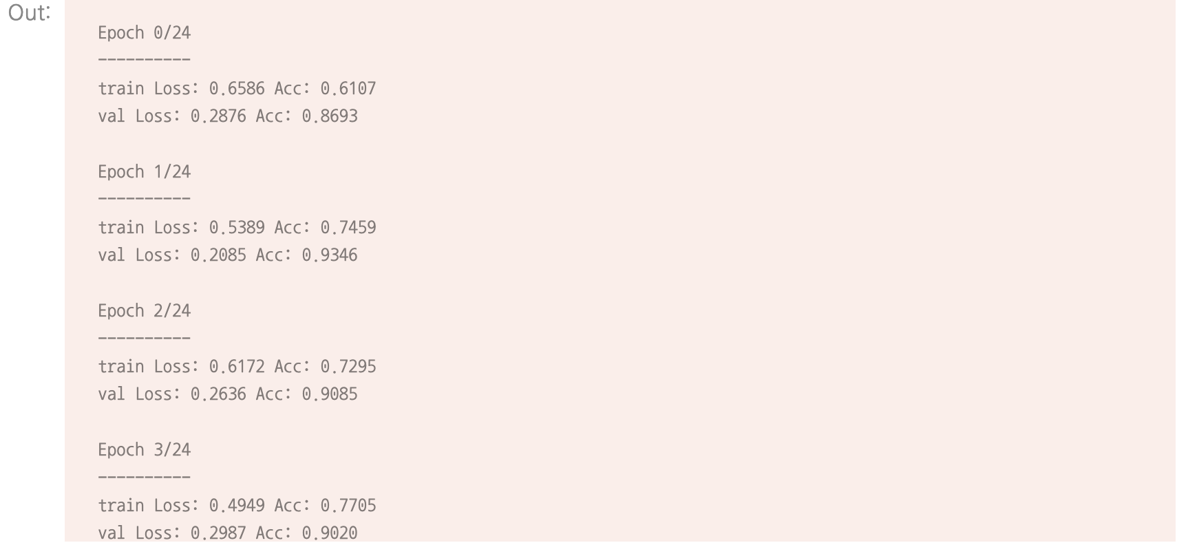

visualize_model(model_conv)

plt.ioff()
plt.show()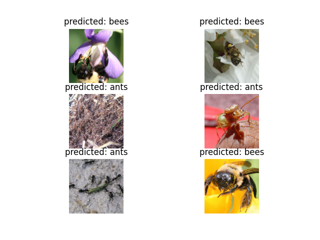

출처 : PyTorch Tutorials https://pytorch.org/tutorials/beginner/transfer_learning_tutorial.html