
I. Implement histogram, KDE, MLE
1. Data (weight-height.csv)
The dataset given in this task consists of columns of gender, height, and weight, and gender is male and female, and height and weight are float data.
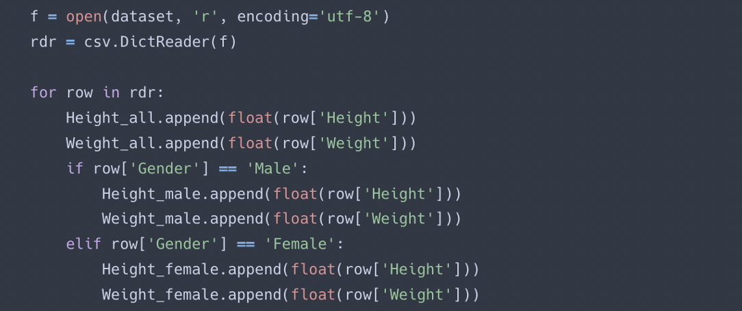
Since the given task needs to load the data and calculate the histogram, KDE, and MLE, the csv file was loaded first. I used Python's csv module to load the dataset, and the csv.DictReader method to read the data in the form of a dictionary. Load the data and store it in a list by dividing it into height all, weight all, height male, height female, weight male, and weight female. The following is a part of the code written to load data.
2. Histogram
The histogram can process data sequentially in a non-parametric method, and has a good effect on visualization, making it easy to understand the data. It is possible to estimate the local density of the histogram, and it is very important to adjust the parameter value for smoothing. Therefore, it is necessary to select a parameter value that is neither too large nor too small for the actual data.
However, the histogram is difficult to apply because the estimated density is discontinuous, and if the D-dimensional data is divided into M bins, the total number of bins becomes M^D, and the computational complexity increases exponentially
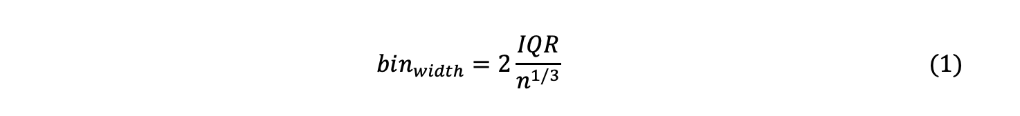
The Freedman Diaconis Estimator was used to find the optimal number of bins, and the upper and lower limits were set as the maximum and minimum values of the data sample. The binwidth is proportional to the interquartile range (IQR) and inversely proportional to cube root of a.size. It is said to perform better on large data sets than on small data sets, and IQR is powerful against outliers.
The following is a part of the tutorial and implemented code referenced for this. (Refer: https://numpy.org/doc/stable/reference/generated/numpy.histogram_bin_edges.html)
3. KDE
Kernel Density Estimation, one of the non-parametric density estimation methods, is a method that improves problems such as discontinuities in histograms by using a kernel function.
First, the kernel function is defined as a non-negative function that is symmetric about the origin and has an integral value of 1, and Gaussian, Epanechnikov, and uniform functions are typical kernel functions. KDE is expressed by the following formula.
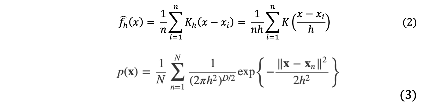
In the above equation, h is the bandwidth parameter of the kernel function, and it is a parameter that controls whether the kernel is in a sharp (small h value) or a smooth (h large value). The probability density function obtained through KDE can also be seen as a smoothing of the histogram probability density function. At this time, the degree of smoothing depends on what bandwidth value kernel function is used as shown in the figure below.
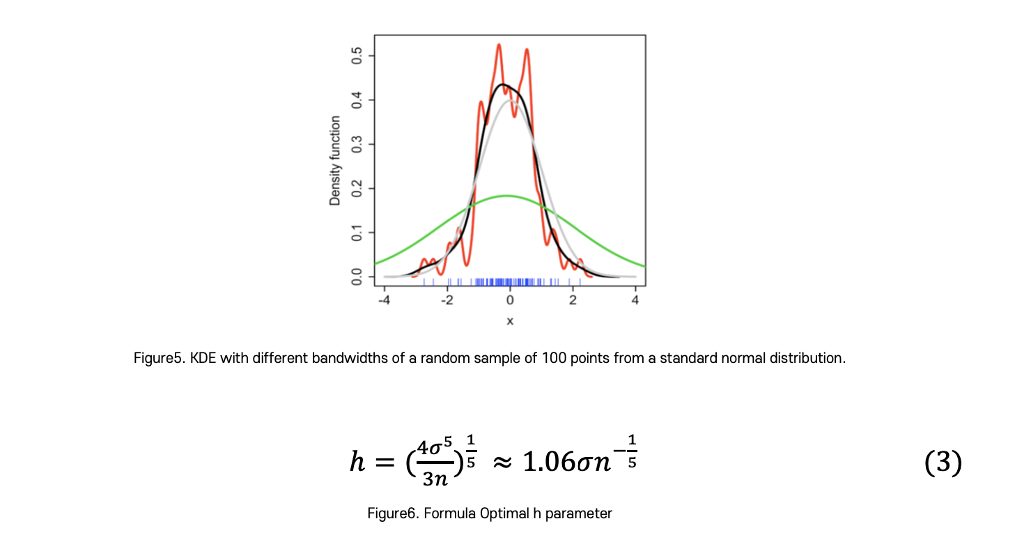
When using the Gaussian kernel function, the optimal bandwidth parameter value is as follows, so I adjusted the H parameter using the above equation. Here, n is the number of sample data and σ is the standard deviation of the sample data.
4. MLE
MLE is a method of selecting a candidate that maximizes the likelihood function (or log likelihood function) among a number of candidates that can be the parameter θ of the assumed probability distribution as an estimator of the parameter.
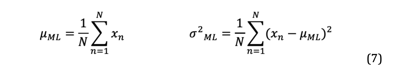
Likelihood refers to the likelihood that the data obtained now come from the distribution. Here parameters were estimated for that data using μML and σ2 ML.
To calculate the likelihood numerically, the likelihood contribution from each data sample can be calculated and multiplied. The reason for multiplying the height is that the extraction of each data is an independent event. As shown in the equation below, the combined probability density function of the entire sample set is called the likelihood function.

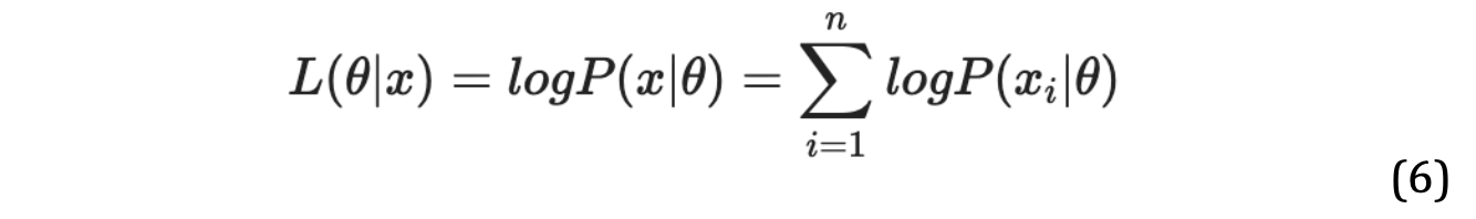
Usually, the log-likelihood function is used as follows, using natural logarithms.
The MLE mean and MLE variance were calculated from the given data sample, and the curve was plotted using the Gaussian distribution function. The MLE shows the trend of a sample of data in a simple shape and describes the optimal approximate distribution. The following equations were use
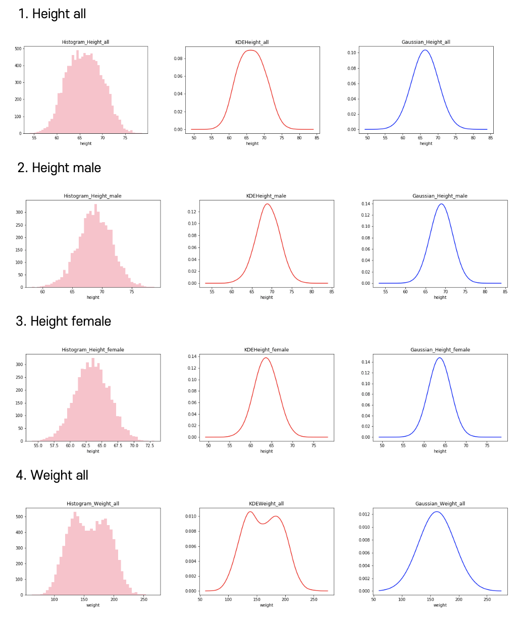
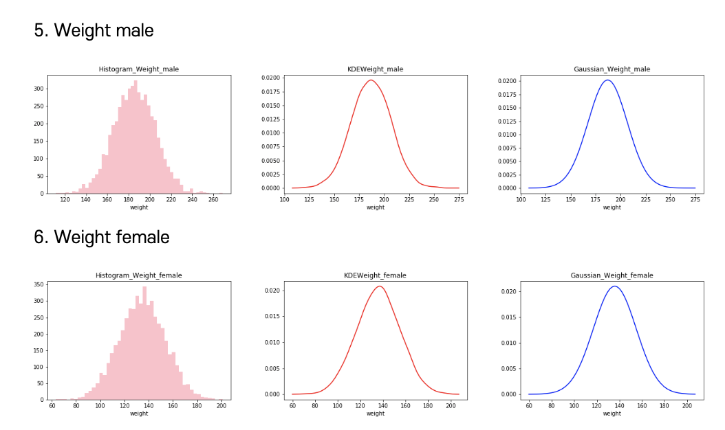
Result
머신러닝 네번째 과제ㅎ_ㅎ 히스토그램도 핑크핑크해