
필요 라이브러리 Import
import pandas as pd
import numpy as np
import matplotlib.pyplot as plt
import seaborn as sns
import warnings
import xgboost as xgb
import shap
from sklearn import preprocessing
from sklearn.preprocessing import OneHotEncoder
from sklearn.preprocessing import LabelEncoder
from sklearn.model_selection import train_test_split
from sklearn.model_selection import GridSearchCV
from sklearn.linear_model import LinearRegression
from sklearn.ensemble import RandomForestRegressor
from sklearn.svm import SVR

warnings.simplefilter(action='ignore')
데이터 불러오기
Data Dictionary
-
id : 선수 고유의 아이디
-
name : 이름
-
age : 나이
-
continent : 선수들의 국적이 포함되어 있는 대륙.
-
contract_until : 선수의 계약기간이 언제까지인지.
-
position : 선수가 선호하는 포지션. ex) 공격수, 수비수 등
-
prefer_foot : 선수가 선호하는 발. ex) 오른발
-
reputation : 선수가 유명한 정도. ex) 높은 수치일 수록 유명한 선수
-
stat_overall : 선수의 현재 능력치.
-
stat_potential : 선수가 경험 및 노력을 통해 발전할 수 있는 정도.
-
stat_skill_moves : 선수의 개인기 능력치.
-
value : FIFA가 선정한 선수의 이적 시장 가격 (단위 : 유로)
Domain
-
Age : 전성기 나이는 보통 27 ~ 29세로, 자기 관리 유무에 따라 25 ~ 31세까지로 보기도 한다.
-
id : data에서 의미하는 것인지는 확실히 모르지만 각 선수의 고유 등번호가 존재하고 이는 명성 또는 잘하는 선수의 척도가 되기도 한다.
-
continent : 아시아쪽 보다 유로파 리그 또는 아메리카 대륙쪽이 축구가 더 발전되어 있는 경우가 많다.
train_data = pd.read_csv("./FIFA_train.csv")
train_data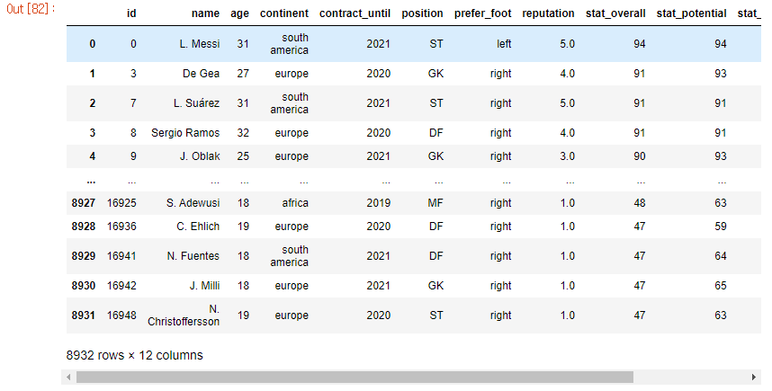
train_data.info() #데이터 자료형 확인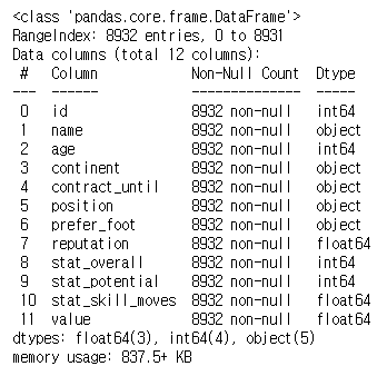
train_data.isna().sum()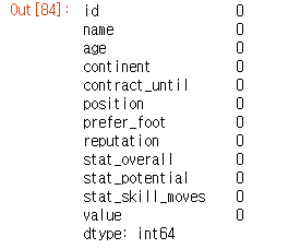
- train_data를 불러와서 자료형 및 결측치 확인
- 결측치가 없는 것을 확인
train_data.describe()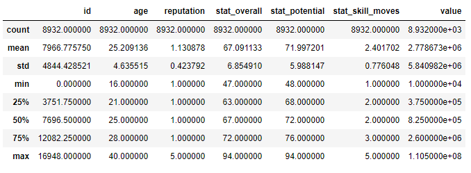
train_data.describe(include=['O']) #범주형 데이터 확인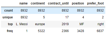
- 각 data의 개수, 평균, 백분위수(수치형 데이터) / 최빈값 등을 확인
train_data.hist(figsize = (16, 12))
plt.show()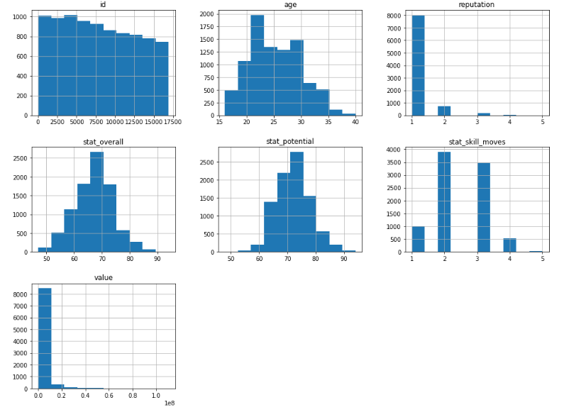
- 수치형 data의 히스토그램을 확인
- stat_overall과 stat_potential이 유사한 형태의 분포를 나타내고 있는 것을 볼 수 있다.
데이터 분석 및 전처리
train_data['continent'].value_counts(ascending = True)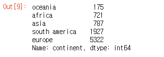
train_data['contract_until'].value_counts(ascending = True)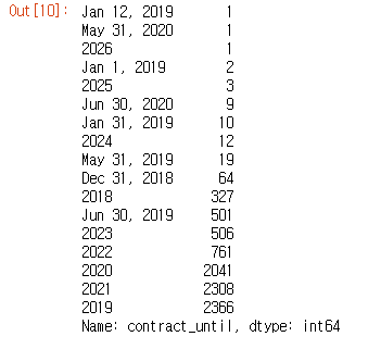
train_data['position'].value_counts(ascending = True)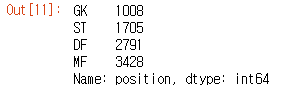
train_data['prefer_foot'].value_counts(ascending = True)
- 전반적으로 각 column에 어떤 수치들이 있는지 확인을 한다.
- contract_until에 년도가 아닌 다른 형태로 값이 들어가 있는 것을 확인하였다.
train_data['contract_until'] = train_data['contract_until'].apply(lambda x : int(x[-4:]))

train_data['contract_until'].value_counts(ascending = True)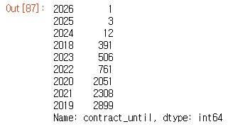
- 해당 년도까지만 나오도록 데이터를 수정하였다.
- 2025년, 2025년은 outlier일 가능성을 염두해두고 추후 모델 진행시 제외하고 진행도 해볼 예정이다.
plt.figure(figsize = (12, 8))
x = sns.heatmap(train_data.corr(), cmap = 'Blues', linewidths = '0.1',annot = True)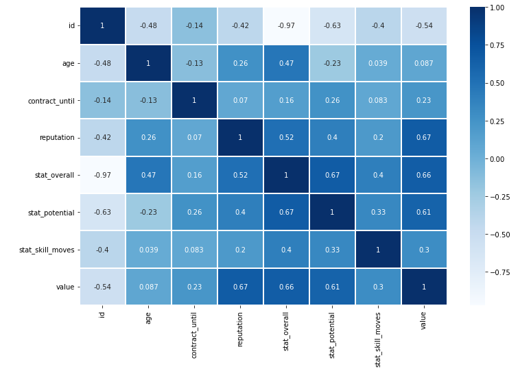
- 각 변수들끼리의 상관관계가 많이 있음을 확인할 수 있다.
- target인 value와 확인해보면 id, reputation, stat_overall, stat_portential이 높은 상관관계를 가지는 것을 볼 수 있다.
f , axes = plt.subplots(2,3)
axes = axes.flatten()
f.set_size_inches(20,10)

sns.barplot(x="continent", y="value", data=train_data, ax=axes[0])
sns.barplot(x="prefer_foot", y="value", data=train_data, ax=axes[1])
sns.barplot(x="position", y="value", data=train_data, ax=axes[2])
sns.barplot(x="reputation", y="value", data=train_data, ax=axes[3])
sns.barplot(x="stat_skill_moves", y="value", data=train_data, ax=axes[4])
sns.barplot(x="contract_until", y="value", data=train_data, ax=axes[5])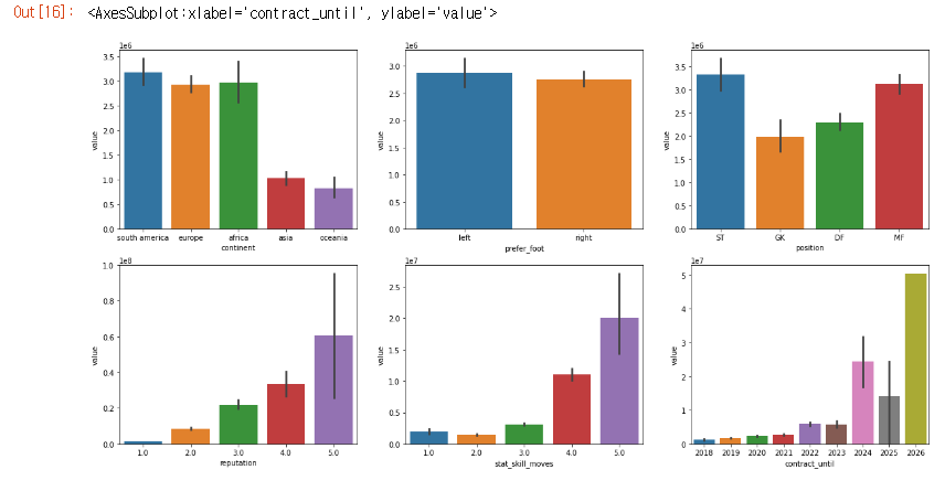
continent
- 인구 순위와는 관계가 크게 없지만 두 분류로 나눌 수 있다.
prefer_foot
- 왼발잡이 선수가 조금 더 많은 연봉을 받는다.
position
- 공격수가 연봉이 제일 높고 다음으로 MF - DF - GK 순서이다.
reputation
- 명성이 높을수록 연봉이 높다.
stat_skill_moves
- 1, 2가 아니면 순차적으로 연봉이 높다.
contract_until
- 연봉이 높은 선수는 이미 오래 계약한 선수들이다.
ax = plt.subplots(figsize=(12, 6))
ax = sns.barplot(x="stat_overall", y="value", data=train_data)
plt.show()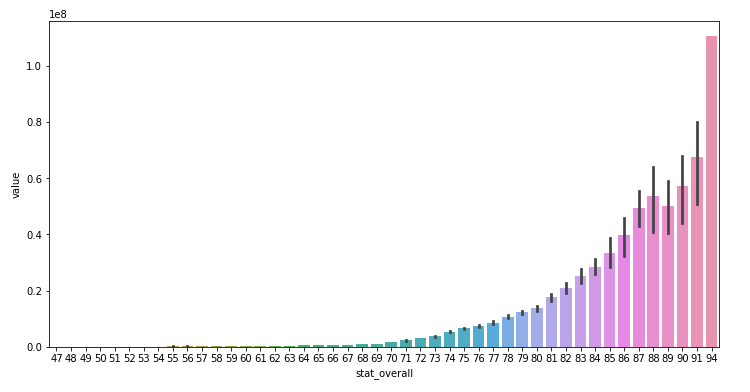
- 전반적인 stat이 높을수록 연봉을 높게 받는다.
ax = plt.subplots(figsize=(12, 6))
ax = sns.barplot(x="stat_potential", y="value", data=train_data)
plt.show()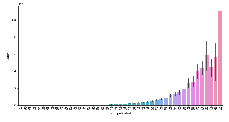
- 잠재적인 stat이 높을수록 value값이 높다.
ax = plt.subplots(figsize=(12, 6))
ax = sns.regplot(x="id", y="value", data=train_data, fit_reg=False)
plt.show()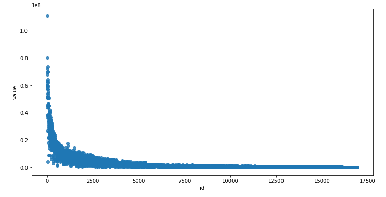
- id가 초반인 선수의 value가 높아지는 경향성이 있다.
ax = plt.subplots(figsize=(12, 6))
ax = sns.regplot(x="reputation", y="id", data=train_data, fit_reg=False)
plt.show()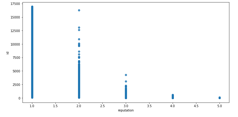
- reputation과 확인해본 결과 어느정도 id와 등번호를 비슷하게 생각하면 될 것 같다는 생각을 하였다.
sns.scatterplot(data = train_data, x = 'stat_overall', y = 'stat_potential', hue = 'stat_potential')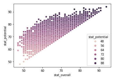
sns.scatterplot(data = train_data, x = 'stat_skill_moves', y = 'stat_potential', hue = 'stat_potential')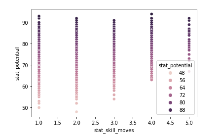
sns.scatterplot(data = train_data, x = 'stat_skill_moves', y = 'stat_overall', hue = 'stat_overall')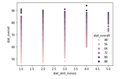
- skill/stat에 관련한 항목끼리 묶어서 확인한 결과 전반적으로 유사한 그래프를 보인다.
train_data.drop(['name'], axis = 1, inplace = True)
cont_index = train_data[train_data['contract_until']>=2025].index
train_data.drop(cont_index, inplace = True)
train_data = pd.get_dummies(train_data)
train_data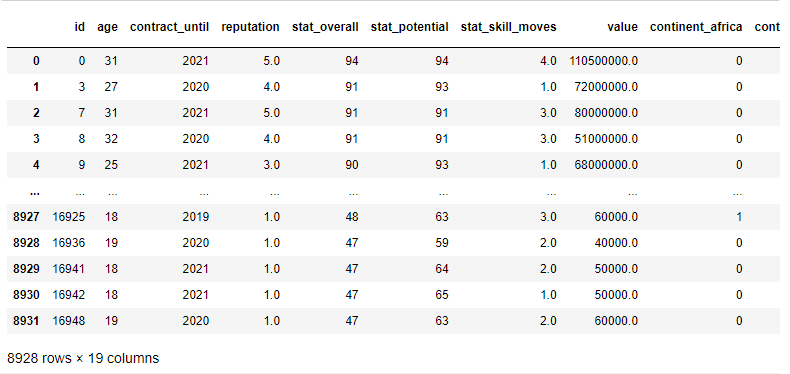
- name은 필요가 없을 것 같아 drop을 하였고, 이전의 outlier라고 생각한 항목은 drop을 하였다.
- 이 후 one-hot encoding을 진행하였다.
scaler = preprocessing.MinMaxScaler()
normalized_data = scaler.fit_transform(train_data)
col = ['id', 'age', 'contract_until', 'reputation', 'stat_overall', 'stat_potential', 'stat_skill_moves', 'continent_africa', 'continent_asia', 'continent_europe', 'continent_oceania', 'continent_south america', 'position_DF', 'position_GK', 'position_MF', 'position_ST', 'prefer_foot_left', 'prefer_foot_right']
normalized_df = pd.DataFrame(normalized_data, columns = col)
normalized_df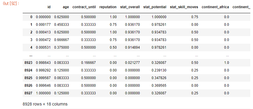
- MinMaxScaler를 이용하여 각 column에 대해 feature scaling을 진행하였다.
모델 적용
y_target = normalized_df['value']
x_data = normalized_df.drop(['value'], axis = 1)

x_train, x_test, y_train, y_test = train_test_split(normalized_df, y_target, test_size = 0.2, random_state=42)

print(x_train.shape, x_test.shape, y_train.shape, y_test.shape)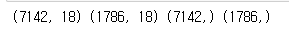
- target을 정한 뒤, train_test_split을 이용하여 train/test data를 분리하였다.
params ={
    'n_estimators':[50, 100, 200, 300],
    'max_depth':[6, 8, 10, 12],
    'min_samples_leaf':[8, 12, 16],
    'min_samples_split':[4, 8, 16, 20]
}

rfr = RandomForestRegressor()
grid_cv = GridSearchCV(rfr, param_grid=params, cv=2, n_jobs=-1)
grid_cv.fit(x_train,y_train)

print('최적 하이퍼 파라미터: ', grid_cv.best_params_)
print('최고 예측 정확도: {:.4f}'.format(grid_cv.best_score_))
- randomforestregressor() 모델을 이용하였고, GridSearch를 이용하여 하이퍼파라미터 튜닝을 하였다.
# 모델 학습
model = RandomForestRegressor(n_estimators = 50, max_depth = 10, min_samples_leaf = 8, min_samples_split = 8, random_state=42, oob_score=True)
model.fit(x_train, y_train)

pred = model.predict(x_test)

# 평가
print("훈련 세트 정확도: {:.3f}".format(model.score(x_train, y_train)) )
print("테스트 세트 정확도: {:.3f}".format(model.score(x_test, y_test)) )
print("OOB 샘플의 정확도: {:.3f}".format(model.oob_score_) )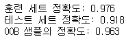

안녕하세요 :) Data/AI 공부 중인 한국외대 컴퓨터공학부 조권휘입니다.